Genetic mapping and manipulation: Chapter 2-Two-point mapping with genetic markers^*

The basics. Two-point mapping, wherein a mutation in the gene of interest is mapped against a marker mutation, is primarily used to assign mutations to individual chromosomes. It can also give at least a rough indication of distance between the mutation and the markers used. On the surface, the concept of two-point mapping to determine chromosomal linkage is relatively straightforward. It can, however, be the source of some confusion when it comes to processing the actual data based on phenotypic frequencies to accurately determine genetic distances. It is also worth noting that most researchers don't bother much with exhaustive two-point mapping anymore. Once we've assigned our mutation to a linkage group, it's generally off to the races with three-point and SNP mapping methods, as these will almost always be necessary to clone our genes anyway. It is worth noting, however, that high-throughput methods for two-point mapping using SNPs (also see below) have been used successfully by some groups and can provide a very precise map position for mutations. These methods may even (in some cases) allow for the molecular cloning of mutations in the absence of further three-point or SNP mapping (Wicks et al., 2001; Swan et al., 2002). Nevertheless, the vast majority of researchers still use the standard tiered cloning progression for which two-point mapping is simply step one.

In carrying out two-point mapping, one can use either genetic or SNP markers. For the purpose of this section, we will cover the use of genetic markers, as the principals are the same and may be somewhat easier to grasp. Often we will carry out traditional two-point mapping using strains that contain two adjacent chromosomal markers, as the strains generated by these crosses can potentially be used later for three-point genetic mapping.

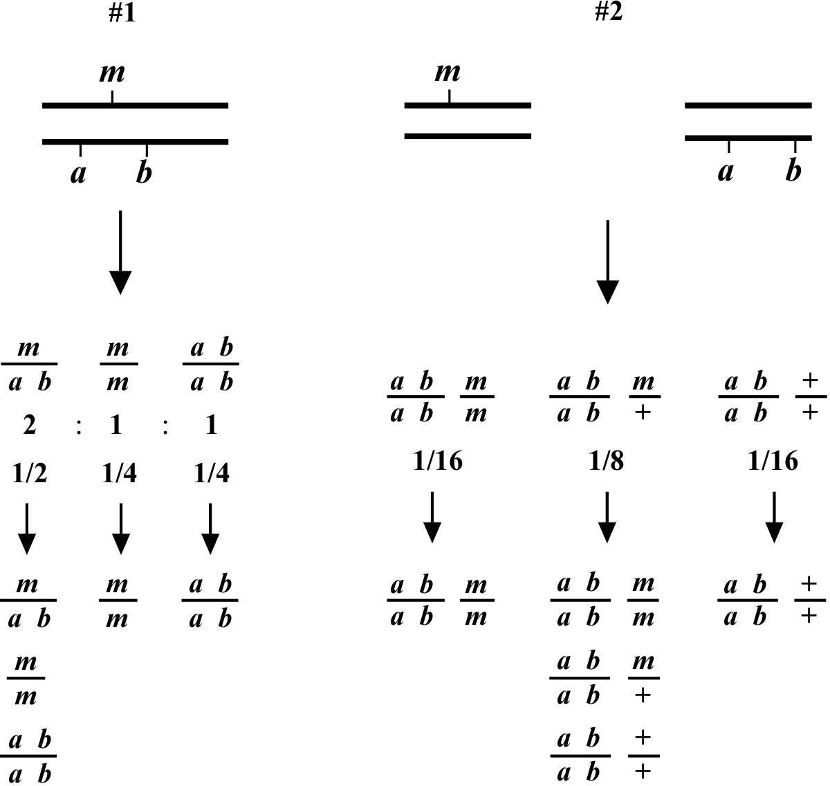
The two most basic outcomes for two-point mapping are shown in (Figure 1). In outcome #1, the chromosomal position of the affected gene (mutation) happens to be on the same/homologous chromosome as the markers being tested. In this case, the mutation is actually flanked by the markers to produce a reasonably well-balanced strain. The genotypes of the progeny are indicated along with the ratios (or fractions) of their occurrences. Three genotypes are generated (m/a b, m/m, a b/a b) with three corresponding phenotypes (wild type, M, A B). In this situation we essentially never see the appearance of the triple mutant phenotype MAB, as this would require an exceedingly rare double-recombination event to take place. Furthermore, if we were to pick animals of phenotype M and examine their self-progeny, we would never see M A B animals. Likewise, A B animals will also fail to segregate M A B progeny. Finally, wild-type animals will always throw both M and A B along with wild-type animals. Seeing segregation patterns of this type tells us that m and a b reside on the same chromosome and also that m resides close to or in between the markers a and b. In the circumstance that the M phenotype is lethal, this may be a useful strain for maintaining m as a balanced heterozygote. Namely, by isolating wild-type segregants at each generation, we can propagate the mutation with relative ease. In addition, this strain can be used for three-point mapping.

In contrast, the situation depicted in scheme #2 shows m and a b on distinct chromosomes. In the first generation, we therefore already expect to see 1/16 of the progeny displaying the triple-mutant phenotype M A B. In addition, if we specifically pick A B animals from this generation, 2/3 will throw M A B progeny. If necessary, draw out all the possible genotypes and corresponding phenotypes to convince yourself that these numbers are correct. Observing these kinds of segregation patterns indicates that the mutation and the markers are on different chromosomes. Another possibility is that the mutation resides on one of the ends of the chromosome (see below). If necessary, these two possibilities can usually be resolved by scoring more animals. In general, basing linkage designation on a small number of data points (fewer than 20) should be avoided.

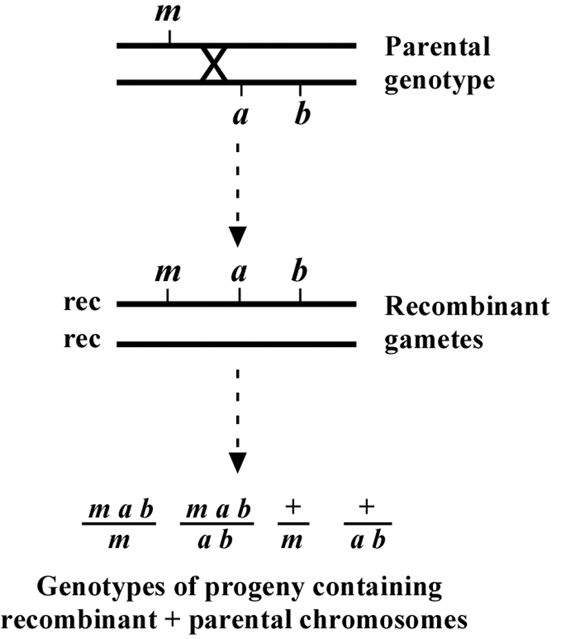
The genetic patterns described above are for the ideal situation where there is no ambiguity in the determination of chromosomal location. But what happens when the mutation lies to one side of the markers, perhaps at some distance? As shown in Figure 2, if the mutation lies to one side, a cross over may occur that will lead to the creation of the two recombinant chromosomes shown. One recombinant chromosome will now contain all three mutations in cis, whereas the other is completely wild type. Also shown are the genotypes occurring when such a recombinant chromosome is paired with one of the parental chromosomes. Now we have a situation where an animal of phenotype M or AB can throw MAB animals. In addition, a wild-type animal can now fail to throw both M and AB animals. In thinking about this, keep in mind that these "rare" recombinant chromosomes will usually - by chance - wind up paired with one of the non-recombinant parental chromosomes in a fertilized zygote. Of course, the farther the mutation is from the markers, the higher the proportion of recombinant chromosomes in the pool, and the greater the possibility that any two recombinant chromosomes may end up together in a zygote.

In these situations we must be careful not to hastily conclude that the presence of such genotypes automatically means that m and a b are on separate chromosomes. The question is more one of frequency. For example, if m and a b are 10.0 map units apart, this means that 10% of the gametes produced by the heterozygote will contain a chromosome that experienced a recombination event in this region. Worms are of course diploid, and progeny therefore have a chance to receive such a recombinant chromosome from either the sperm or the oocyte. Given this distance, the frequency with which progeny will inherit two non-recombinant (also called parental) chromosomes is 0.9 × 0.9 = 0.81 or 81%. The chance of progeny receiving two recombinant chromosomes will be quite small, in this case 0.1 × 0.1 = 1%. However, the frequency of progeny receiving one recombinant and one non-recombinant chromosome is 100 - 81 - 1 = 18%. A significant fraction!

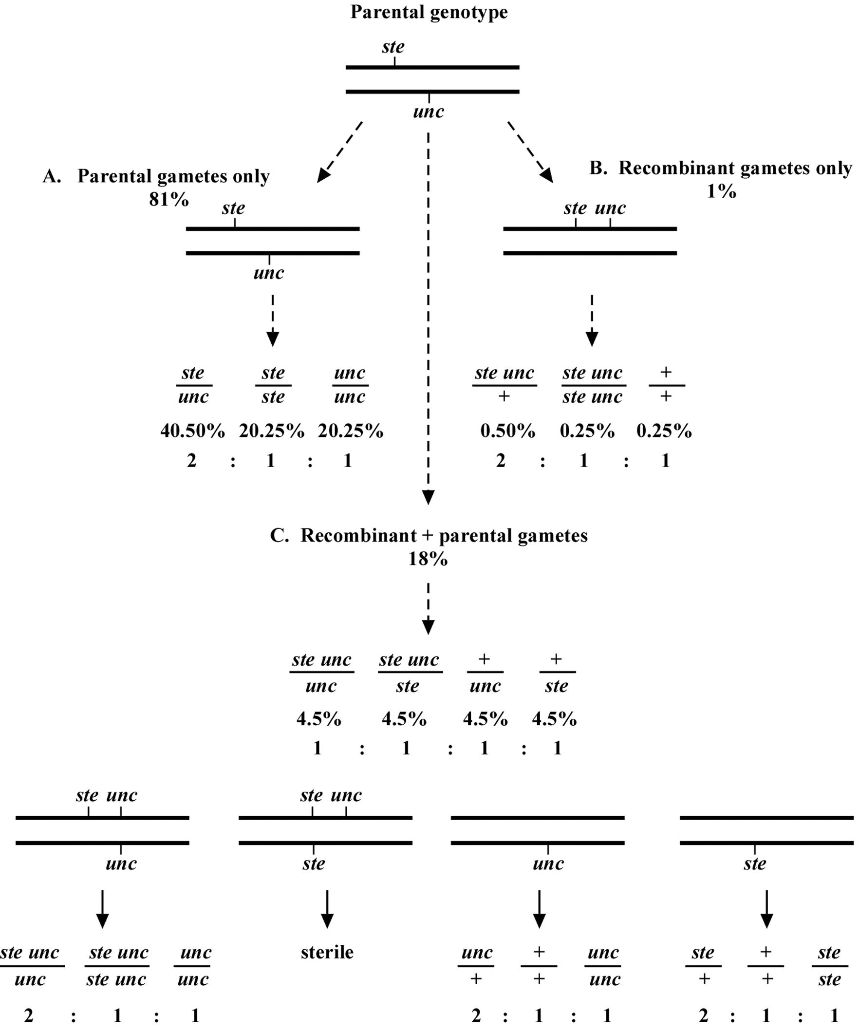
How then do we determine if a mutation is really on the same chromosome as the markers, and if so, what is the distance? This depends in part on how we are doing the mapping. Let us consider one specific example of mapping a sterile (ste) mutation relative to an unc mutation. In the example given in Figure 3, the ste and unc mutations are 10.0 map units apart. Again, this means that 90% of the gamete chromosomes will be of the parental type and 10% will be recombinant. As just stated, the chance of a progeny receiving two non-recombinant chromosomes will be 81% (Figure 3A), two recombinant chromosomes will be 1% (Figure 3B), and one recombinant plus one non-recombinant chromosome will be 18% (Figure 3C).

Of the recombinant chromosomes, one-half (5% of total chromosomes) will be ste unc and one-half (5%) will be wild type (+ +). Each recombinant chromosome has an equal chance of pairing with either of the two parental chromosomes. Therefore, for the animals that contain one recombinant and one non-recombinant chromosome, one-fourth will be ste unc/unc, one-fourth ste unc/ste, one-fourth +/unc, and one-fourth +/ste. These genotypes will therefore be present at a frequency of 0.25 × 0.18 = 0.045 or 4.5% each (Figure 3C).

Now consider mapping in the following way. From plates where the parent is ste/unc, we clone Unc progeny. We want to determine the frequency at which such Unc animals throw Ste Unc versus Unc only progeny. We therefore look for the presence of Ste Unc animals in the next generation. We know that there will be two genotypic possibilities for animals with an Unc phenotype, unc/unc, where both chromosomes are parental, and ste unc/unc, where we have one of each. The percentage of animals with the unc/unc genotype is 0.81 × 0.25 = 0.2025 (20.25%), as 81% will have only parental chromosomes and of these, one-fourth will receive two unc chromosomes. The percentage with a ste unc/unc genotype will be 0.18 × 0.25 = 0.045 (4.5%), as 18% of progeny will have one recombinant and one parental chromosome and there is a 25% chance of receiving both the ste unc and the unc chromosome (0.5 × 0.5 = 0.25). The overall percentage of animals with an Unc phenotype will therefore be 4.5 + 20.25 = 24.75%. Finally, the percentage of Unc animals with a ste unc/unc genotype will be 4.5/24.75 = 18.2%.

The above determination tells us that if our mutation and marker(s) are 10.0 map units apart, we should expect to see about 18% of the cloned Uncs throwing Ste Unc progeny. Similar calculations can be carried out for various genetic distances. To facilitate these determinations, the formula (1-p)(1-p)/4 (where p is the map distance expressed as a fraction; e.g., 10 map units = 0.1) can be used to calculate the predicted fraction of unc/unc animals, whereas the fraction of ste unc/unc animals can be calculated using the formula 2p(1-p)/4. The total sum of these two products will give the fraction of all Unc animals, and the relative percentage of recombinant genotypes (ste unc/unc) can be obtained by dividing the fraction of ste unc/unc animals from the total sum. For example, if the marker and mutation are 1.0 map unit apart, we will see Ste Unc animals appearing from ~ 2% of the cloned Uncs. At 5.0 map units apart, it will be ~ 9.5%; at 25.0 map units, ~40%. The general rule is that when mapping by this strategy, the frequency of animals containing the recombinant chromosome will be about double that of the map distance between the marker and the mutation. As the distance between the mutation and marker increases, this frequency decreases.

Interestingly, by the time we get to 50.0 map units, 67% or 2/3 of Unc animals will throw Ste Unc progeny. This latter number should sound familiar; it's the same percentage you would get if the ste and unc mutations were on separate chromosomes. In fact, at 50.0 map units or greater, two mutations will appear to be unlinked. This usually is not an issue because we tend to carry out two-point mapping with markers at the chromosome center, guaranteeing distances no greater than about 25.0 map units.

There are often multiple ways to carry out two-point mapping using the same set of markers. For example, in the previously described cross we could have picked wild-type rather than Unc animals and looked for the absence of either Unc or Ste animals in their progeny, signifying a + + or wild-type recombinant chromosome. If the marker and mutation are 10.0 map units apart, we will predict to have 0.81 × 0.5 = 40.5% of animals with an unc/ste genotype. We will also have 0.18 × 0.5 = 9% of animals with either an unc/+ or ste/+ genotype (4.5% each). Thus we predict that 9.0/49.5 = 18.2% of the wild-type animals we pick will fail to segregate either Unc or Ste progeny. These numbers are identical to those previously calculated for picking Unc progeny and looking for Ste Unc in the next generation.

Consider this final case however. Imagine you are trying to map an embryonic lethal mutation (emb) relative to a known unc. The easiest way to do this would be to pick wild-type animals from an emb/unc parent and then look for the absence of Unc animals in the progeny (embryonic lethals are usually difficult to score directly by their plate phenotype). If the unc and emb are on the same chromosome and close, very few phenotypically wild-type animals will fail to throw Unc (as well as Emb) progeny. To calculate the map distance, however, we must realize that using our methods, unc/+ animals will not be among those counted as "recombinants" (those wild-type animals that fail to throw Uncs). Thus, if the distance between the unc and emb is 10.0 map units, we predict to have 0.81 × 0.5 = 40.5% animals of genotype emb/unc. We will also have 0.18 × 0.25 = 4.5% of animals with an emb/+ genotype and 4.5% with an unc/+ genotype. Therefore, when picking among the phenotypically wild-type animals, the frequency of emb/+ animals will be 4.5/(40.5+4.5+4.5) = 9.1% (and not 18.2%) of the total. Being aware of these factors and, as always, drawing out the cross carefully will prevent interpretive errors. For a discussion of additional two-point mapping strategies as well as potentially useful formulas for correlating map distances with phenotypes, see Hodgkin (1999).

A question of strategy: To map all chromosomes at once or to do so sequentially? This may depend on several factors such as time constraints and competitive pressures. Everything being equal, mapping sequentially is the most efficient allocation of time because once one has positively identified a chromosomal location, one need not check all the other chromosomes. In practice though, we often want to map our mutants as quickly as possible and will test multiple chromosomes at once. In addition, the presence of clear negative data can strengthen conclusions when the mutation lies at some distance from the markers. Along these lines, it is worth noting that a number of strains containing markers for multiple chromosomes have been generated for the express purpose of enhancing mapping efficiency. For example, strain MT464 contains the markers unc-5, dpy-11, and lon-2, thereby permitting the simultaneous mapping of chromosomes IV, V, and X, respectively.

It is also worth pointing out that an observant experimentalist can often get a good sneak peak at what the three-point data will ultimately confirm during the two-point mapping process! In fact, this is another good reason to carry out two-point mapping using adjacent markers. To reiterate, we already know that if the mutation (m) happens to be on the same chromosome as the markers a and b, then the large majority of M animals coming from the heterozygous parent (m/a b) will fail to throw A B progeny. Because of recombination, however, you may observe a small percentage of M animals throwing either M A, M B, or M A B animals. For example, if you happened to observe three plates (out of 25) with M A B animals and one plate with M A animals, that would suggest that m lies to right of b and is at some distance from the markers. In contrast, if you were to only observe several plates with M A animals, m would be likely to lie to the right of b but close to the markers (or perhaps between them and just to the left of b). If M A B animals are never observed but there are a small percentage of M A and M B animals, then m must lie between the markers. If this reasoning is not yet clear, read over the three-point mapping chapter and then come back and draw this out to confirm the predictions. This bonus gift of two-point mapping can be a real time saver.