 Embryo series courtesy of Einhard Schierenberg
Table of Contents
Welcome to the world of C. elegans genetics. The field has historically used classical genetic methods for two principal purposes: (1) to define precisely the locations of mutations so that the affected gene products can be identified, and (2) to generate strains containing multiple mutations or visible markers for genetic and phenotypic analysis. The following sections will address both concerns, although much of the emphasis is admittedly placed on the genetic mapping of mutations. Practically speaking, however, there is little distinction between these two categories. Many or all of the principles relevant to standard genetic analysis are integral to the mapping process and strains generated as biproducts of genetic mapping typically facilitate subsequent genetic and functional studies.
The actual process of genetic mapping and mutant gene identification has evolved dramatically since the first C. elegans mutants were cloned in the late 1970's and early 1980's. In fact, the process of mutant gene identification in C. elegans has undergone a major shift in recent years. New rapid genome sequencing methodologies have made it possible to dramatically reduce efforts previously spent on the positional mapping of mutants (Sarin et al., 2008; reviewed by Fay, 2008; and Hobert, 2010), an issue that is addressed in more detail at the end of this section. Thus, the question arrises, is classical genetic mapping destined to go the way of the dinosaurs, knitted-neon leg warmers, or quoting Borat? In short, the answer is not entirely. Standard genetic procedures will continue to play an important role in the identification of mutants and for generating useful reagents for biological analysis. The principle difference will be one of degree, and this is good news for everyone.
Note that some of the following sections contain material discussed in greater detail in other sections of WormBook such as Maintenance of C. elegans. Also, for these sections to be nominally useful, readers will need to possess a basic working knowledge of Mendelian genetics. Finally, for a concise review of some of the topics discussed, see Hodgkin (1999).
Genetics has its good and bad points. On the positive side, in the hands of a competent researcher, genetics typically works, producing interpretable and internally consistent results. This may lead us to our goal of cloning mutations from genetic screens or may enable us to create complex configurations of mutations in order to uncover meaningful functional relationships. In this sense, it can be quite satisfying, particularly if we have been clever and creative in the process. On the down side, genetics can sometimes seem like a slow and arduous progression, and we are often “slaves” to the developmental timeclock of the worm. Moreover, even when a reasonably careful approach is taken, genetics can sometimes fail to provide a clear answer. For example, we may generate pieces of conflicting data that must be resolved by additional experiments.
Being a successful geneticist (not to mention scientist) requires a high level of foresight, diligence, and commitment. Half measures and vague notions will seldom suffice. Unlike coursework, there is generally no partial credit in the real world of science. One faulty link in the chain of logic and experimental execution usually leads to zero results. The three keys to success in genetics are as follows: (1) understand from the start exactly what you are doing and what you expect to happen at each step, (2) notice if things do not go as expected, and (3) always take the patented “sledgehammer” approach. The bottom line is that to be an effective C. elegans geneticist you must consistently get things to work the first time. Failure to do so will vastly reduce your progress. In this sense, C. elegans genetics is not substantially different from many other scientific disciplines. Given the time required for worms to develop, however, one can waste significant time and effort before discovering that the experiment has failed. Try hard to prevent this from happening to you.
To ensure the first point—thoroughly understanding your experiment from beginning to end—it will almost always be necessary to draw out the entire set of crosses, taking into account and quantifying all possible outcomes. This is particularly true when you are just starting out in genetics, and you will want to do this before picking a single worm. Remember this: if your basic strategy is flawed, then all the experimental diligence in the world won't save you. Each genetic situation will have unique considerations. By sketching out the entire genetic flowchart, complete with all possibilities, one can nearly always guarantee a good result. Avoid at all costs a faulty scheme. DRAW IT OUT!
With respect to the second point, it is essential that you quickly and consistently note any inconsistencies between the expected results and those actually obtained. This requires looking hard at your plates over the entire course of the genetic procedure. Continually ask yourself if the observed plate phenotypes make sense and if the approximate ratios are in line with your expectations. Do not sweep any significant inconsistencies under the rug! This is a red flag and may be telling you that either one of your starting strains is not as advertised or that there is a fundamental error in your experimental design. Both situations are your responsibility to avoid. Bad or incorrectly described strains can generally (though not always) be detected by a careful examination of the strain before beginning the experimental process. Rather than investing weeks or months of your time in trying to work with a questionable strain, obtain (or generate) a correct version of the strain from some other source, or possibly come up with an alternative strategy for your experiment. Sometimes it may be difficult or impossible to know if a strain is definitively correct. To some extent we must operate on faith, and we are usually safe in doing so. It is always advisable, however, to have multiple pieces of corroborating data before moving on to subsequent steps, particularly when it comes to genetic mapping.
Finally, always take the “sledgehammer” approach. The bottom line is that it usually takes only a couple of extra minutes to pick a few more animals or to set up additional plates for matings. Contrast this to the days or weeks that can be lost if sufficient animals were not picked to isolate the necessary genotype or generate sufficient numbers of crossprogeny. Plates are cheap, but your time is precious.
This is in many ways the bane of all genetics and why non-geneticists typically deplore reading our papers. The problem is that the style and rules of nomenclature are different for all the commonly studied organisms. Moreover, unification between the fields is unlikely ever to occur as we are too entrenched in our unique notations and jargon. The general rules for C. elegans are described below. Additional information can be found in Maintenance of C. elegans.
These are designated by three letters followed by a hyphen and a number. The letters and number are always italicized. The letters chosen are usually either abbreviations of a longer descriptor (such as lin for lineage defective or unc for uncoordinated) or may be acronym-like (such as sur for suppressor of ras). A number then follows the letters (such as lin-31) to indicate the approximate order in which the mutations were discovered.
Originally, most or all gene names were derived from genetic screens in which mutant alleles were isolated. In some cases the actual open reading frame (ORF) that is compromised in these mutants may still await identification. Subsequent to the sequencing of the worm genome, many names have been given to ORFs (or predicted ORFs) for which no mutations have been identified. This most often occurs when an ORF is homologous to one or more genes characterized in other systems or when an ORF encodes for a conserved peptide motif, thereby implicating it is a member of an extended gene family.
There is something of a protocol in our field that should be followed before assigning one's favorite new mutation a novel three or four-letter name. First, efforts should be made to initially map the mutation, in part to prevent the assignment of a new name to a previously described mutation or gene. For a number of good reasons, it is becoming quite common now for genes to be cloned (the mutant ORF positively identified) before assigning gene names. If the gene or mutant is believed to be novel, a proposed name is submitted to the “worm gene czar”, currently Tim Schedl, who then passes sound judgment on the merits of the suggested acronym.
This is both simple and confusing: simple because the name of a mutant strain, lin-31 for example, is the same as the name of the gene affected in this strain, lin-31, and confusing because when we say ”lin-31“ we may mean either the (wild-type) ORF that encodes lin-31 or mutant lin-31 animals. Obviously the context will specify which definition is meant. When we refer to a specific mutation that affects lin-31 function, we often tack on to the end an allele designation. These are commonly one or two letters (usually two) followed by a number, such as the allele lin-31(n301). The letters that proceed the number are specific to each C. elegans lab or principal investigator and allow one to identify the origin of the mutant allele (n for example is the Horvitz lab's designation). Allele numbers correspond to the order in which they were identified by a given lab. Of course, the nature and severity of the mutant phenotypes displayed by individual alleles for any given gene may vary greatly.
The peptide encoded by lin-31 is LIN-31.
More complexity. When describing the phenotype of an animal, we capitalize the first letter and do not use italics. Thus animals with an unc-4 genotype display an Unc phenotype. In addition, such animals may display other defects, for example they may be slightly small, or Sma. With time one gets to know all the major descriptors, which isn't really too onerous a task given that there are only a limited number of ways to really mess up a worm.
Below is a list of the most common types of marker mutations used for standard genetic mapping. One issue to always consider is the penetrance of the allele. If the penetrance is significantly below 100%, the marker may be difficult or even impossible to use for mapping. Another issue is the ease with which the mutation can be scored by its plate phenotype. Wormbase provides information about specific mutations and alleles. A scale of one to three (ES1, ES2, ES3) is commonly used to designate the ease of scoring of the plate phenotype. ES3 mutations are generally very easy to score, whereas most ES1 mutations require some level of clairvoyance and a pair of dowsing rods (Sigma catalog #DR502). ES2-rated mutations range from the reasonable to the ridiculous. For a more complete listing of mutants and phenotypes, see Wormbase.
dpy Dumpy (Dpy); short and fat phenotype. Different dpy mutants can range from severe (small footballs) to moderate (slightly pudgy) in character. The more severe ones will often display a variable Unc phenotype as well.
unc Uncoordinated (Unc). There are many different subclasses of unc mutants. These include coiler Uncs, kinker Uncs, paralyzed Uncs, shrinker Uncs, Uncs that fail to move backwards when touched with a pick on their heads, Uncs that display poor forward movement but back well, etc. Recognizing certain types of Uncs can initially be challenging, although it usually gets easier over time. Often Uncs are somewhat misshapen and are typically smaller or thinner than wild-type animals.
sma Small (Sma). These animals tend to be more proportional in shape than Dpy animals; less stocky, more like wild type.
lon Long (Lon). These animals can often be a bit on the thin (stringy) side. Although Dpy and Sma animals can in some cases be very small as compared with wild type, even the longest Lon is only about 50% greater in length than wild-type animals.
egl Egg-laying defective (Egl). This can lead to the Bag (bag of worms) phenotype where embryos hatch within the mother, leaving a cuticle sack containing multiple wriggling larvae. Egl animals can be recognized prior to bagging as adults that appear bloated with eggs. Caution must be used, however, as aging wild-type hermaphrodites can often appear somewhat Egl over time. An individual bag will only last for about 24 hours (at 20 °C) on the plate. Once worms become starved, the incidence of Egls and Bags in genetically wild-type animals increases substantially. Unambiguous identification must always be carried out on non-starved plates.
let Lethals (Let). These can range from embryonic lethals that never hatch to lethals that die as larvae. The latter category is easier to recognize, especially when the worms display a distinct larval lethal phenotype such as a “paralyzed rod” or a severe Dpy. Dead or dying eggs can be difficult to distinguish from healthy wild-type eggs on first viewing with a dissecting scope. To “see” embryonic lethals, one must allow a parent to lay eggs for a set period of time (usually 3-12 hours). The parent is removed to a new plate, and the fates of the eggs are followed. The presence of lethals can usually be identified unambiguously after about 18 hours (at 20 °C) when the vast majority of wild-type embryos would have already hatched. Other designations for embryonic lethal mutations include emb and zyg.
ste Sterile (Ste). These animals come in several varieties. The most useful for mapping are those in which the sterility is obvious because the adult worms are devoid of eggs. Care must be taken to avoid mistaking a sterile animal for one that is merely a young adult that does not yet contain obvious eggs. If in doubt, transfer the suspected sterile animal to a new plate and follow its fate. In some cases, sterile animals may contain a protruding vulva (Pvl-sterile), which makes identification facile. So called “maternal-effect” lethal mutants are really just sterile animals that contain dead eggs and are therefore harder to recognize.
rol Roller (Rol). Animals form a horseshoe shape and tragically twist in place about their long axis. The Rol phenotype can be masked by strong unc or dpy mutations, which prevent the animals from carrying out the classic roller moves.
bli Blister (Bli). Adult animals have a variably blistered cuticle, which can resemble a large bubble on the surface of the worm. The Bli phenotype can be suppressed by a number of dpy and rol mutations.
lin Lineage defective (Lin). These can display any number of distinct defects in the pattern of cell divisions that occur during development. Consult WormBase or other sources for specifics concerning the defects associated with particular mutants.
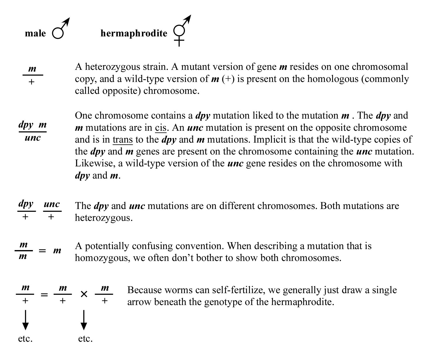
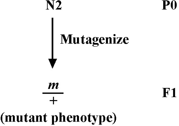
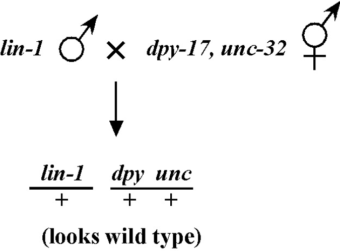
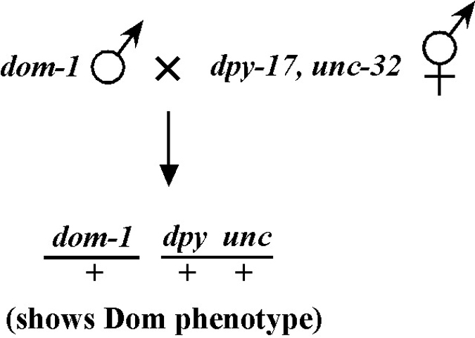
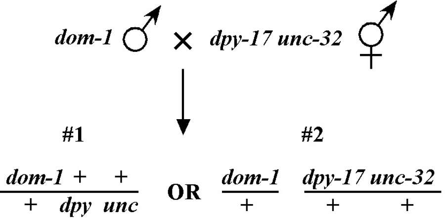
There are undoubtedly numerous “correct” ways to convey genetics in writing. Some standard C. elegans conventions that I use throughout the sections are shown in Figure 1.
Maintaining a worm stock is usually relatively straightforward. Worms are typically grown on Nematode Growth Medium (NGM) plates containing the bacterial (E. coli) strain known as OP50. They crawl around the plate, eat off the bacterial lawn, and reproduce. The plates are secured with a rubber band and are stored upside down to prevent them from drying out. Usually worms are grown at either 15 °C or 20 °C. It takes about 3.5 days at 20 °C for a fertile adult to develop from a one-cell embryo. At 15 °C this process takes about twice as long, and varying the incubation temperature (between 15 °C and 20 °C) is pretty much the only way to control the rate of worm growth and development. Higher temperatures (20 °C to 25 °C) can further expedite the rate of development but can cause a drop in fertility and poor health, especially in certain mutant backgrounds. Temperatures >25 °C are usually harmful and should be avoided under normal circumstances.
Embryogenesis itself normally takes about 14-16 hours at 20 °C. This is followed by four larval stages during which all growth occurs. Wild-type worms kept at 20 °C will begin producing and laying eggs 3-4 days into their life cycle and will produce on average 220 or more self-fertilized progeny. After about two generations, the OP50 bacteria will be completely consumed, and the worms will become starved. Starvation in worms does not have the same connotation as it might in other organisms. Worms are tough and can survive without food for extended periods of time. They do this in part by forming “dauer” larvae, which are dark and thin and often lie motionless. Neglected worms can survive for up to several months, provided the plates do not become badly contaminated or dry out. Wrapping plates in Parafilm and storing at 10 °C to 15 °C can help to increase long-term survival rates.
It is important to stress that taking a lackadaisical attitude towards ones worms stocks is not to be encouraged. Loss of a precious strain can be exceedingly painful. The time required to regenerate the strain can be costly, and in some instances may not even be possible. Loss of strains may result either from letting the plates get too desiccated (high danger sets in by the fruit leather stage and is extreme by the potato chip stage) or through a fungal or bacterial contamination that is detrimental to nematode survival (also see below). In fact, contamination is a more common cause of strain loss and can occur quite rapidly (< 2 weeks) in the case of particularly nasty infestations (such as the virulent mold we refer to as “the orange death”). It is also important to note that for less-robust strains, survival on even reasonably moist (but starved) plates may be an issue after several weeks. Thus it is essential to check on your strains once a week at the minimum to ensure their long-term survival. In addition, all newly generated or received strains should immediately be frozen away, as this is the only surefire way to “guarantee” that the stock can be regenerated (and that you stay off of Theresa Stiernagle's public List of Shame).
Avoid contamination! There are two general types of contamination, bacterial and mold/fungal. Though the mold (generally a fuzzy growth) may appear especially sinister and will require a fairly rapid response, it is the easier of the two to get rid of. Normally, a mold can be defeated by transferring animals to a clean plate, and then moving them to a second clean plate after several minutes or an hour. Bacterial infestations occur when strains other than OP50 colonize the plate. Getting rid of bacteria can be problematic. This is because the worms have been eating the stuff and it's in their intestines. The only way to get rid of a nasty bacterial infestation is to dissolve gravid (fertile, egg-containing) worms in a mixture of sodium hypochlorite (bleach) and sodium hydroxide; this mixture will kill everything but the internal eggs, which are protected by their chitin shell.
Contamination will come from three sources: (1) the agar plates themselves may harbor embeded seeds of destruction, such as the dreaded exploding “footballs” or some other unwanted microbe; (2) the OP50 used to spot the plates may itself be contaminated; or (3) air-born nasties, which are usually of the fungal or mold-like variety, can fly onto your plates. Obviously, one wants to do everything possible to avoid using inherently bad plates, and a thorough appreciation for sterile technique (not to mention a high level of paranoia) should be instilled in those pouring the plates. Bad OP50 is often due to lack of proper sterile technique. Always inoculate liquid LB cultures by picking OP50 colonies from a reasonably fresh LB plate. Never inoculate a new OP50 liquid culture from a preexisting OP50 liquid stock as this will nearly ALWAYS lead to contaminants. To avoid bad OP50, some labs even transform their OP50 strain with an Amp resistance plasmid, and then grow the liquid culture of OP50 in the presence of ampicillin. Other labs may let a small sampling of spotted plates from each batch sit at room temperature for a week before using the bulk of the plates (stored at 4 °C) to allow any widespread contaminants to manifest themselves. To avoid mold and fungus infestations, keep plates covered whenever possible while picking. Also toss discarded plates into covered bins and periodically inspect your incubators boxes containing ancient plates, which are typically highly contaminated. Basically, use good sense and be meticulous about your plate pouring and spotting techniques. A bad contamination can literally ruin an experiment, kill your strains, or at the very least make the work far less pleasant.
Maintaining a worm stock can be significantly more difficult if the strain is not “balanced”. Roughly speaking, a balanced strain is one that contains distinct mutations on each copy of a particular chromosome. Balancing a mutation is usually an issue only if the mutation causes lethality or sterility when it is homozygous. A sterile mutation, for example, could be balanced by a set of dpy and unc mutations on the homologous chromosome. Usually the best configuration for balancing is when the markers are close together and flank the mutation that needs to be balanced. This decreases the likelihood that the mutation will be lost because of a single recombination event. Still, even having close flanking markers does not guarantee that the strain cannot be lost over time, and diligence must be exercised during each passage of the stock to make sure that this does not occur. Other than having a homozygous mutation, the most stable situation is when the mutation is balanced over a chromosomal translocation or deficiency (see Genetic balancers). In this case, the “balancer” chromosome is homozygous lethal and may also prevent recombination from occurring in the region of the mutation.
C. elegans has six chromosomes: five autosomes (I-V) and one sex chromosome (X). Hermaphrodites are diploid for all six, whereas males are diploid for the autosomes but are haploid for X (designated X/Ø). A variety of visible markers for mapping (such as dpy and unc mutations) are present on all six chromosomes. Although these markers are distributed to some degree along the entire length of the chromosomes, there is a markedly higher density occurring in the central regions of each autosome. For this reason (and others) it has generally been easier to map and clone mutations that reside in the central or “gene cluster” regions of the autosomes. As discussed below, however, the ability to use single nucleotide polymorphisms (SNPs) (see Section 3) for genetic mapping has largely (although not completely) abrogated many of the disadvantages associated with cloning mutations outside the clusters. Moreover, the application of whole-genome sequencing methods is certain to further level the playing field.
During meiosis, the four homologous chromatids (produced by the duplication of each parental autosome) join together to form the structure known as the synaptonemal complex. The exception is the X chromosome in males, for which there are only two chromatids. In general, a single crossover event will occur between just one of the two pairs of parental chromosomes. The pair of maternal and paternal chromosomes that undergo the exchange will consequently contain both maternal and paternal sequences. The other maternal-paternal chromatid pair will remain in their original form. Although this pattern of a single crossover event for each synaptonemal complex is highly reproducible, occasionally both or even neither pair of chromatids will undergo strand exchange. In addition, at low frequencies, two spatially separated crossover events can occur between a single pair of chromatids. When such double exchanges occur, they generally take place at opposite ends of the chromosomes because the crossover points (called chiasmata) somehow discourage other nearby crossover events. The practical consequence of this phenomenology is that we are almost always safe in assuming that the recombinants that we isolate are the result of a single crossover event, particularly if we are targeting crossovers within relatively small regions of the genome.
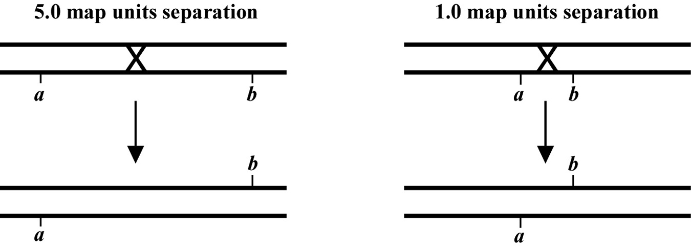
The genetic distance separating two genes (or any two points on a chromosome) is determined by the frequency of meiotic recombination that takes place between them. The nearer the two genes are to each other, the less likely that a recombination event will occur in that span. One (1.0) map unit (also sometimes called a centiMorgan; cM) is equal to a 1% meiotic recombination frequency. In other words, if on average 1% of all gametes (sperm or oocytes) have experienced a recombination event between two particular genes, then these genes are considered to be 1.0 map unit apart. Note that recombination frequency has been reported to change somewhat with temperature and age of the parent. Although the frequency of meiotic recombination does not substantially vary between 16 °C and 20 °C, rates increase significantly at temperatures greater than 20 °C and decrease at temperatures below 15 °C.
In the examples shown in Figure 2, the recombination event on the left will occur in 5% of the gametes whereas the one on the right occurs in 1%. Both lead to mutations a and b becoming genetically (and physically) unlinked from each other. Most chromosomes are on average about 50 map units long. This means that mutations on opposite ends of a chromosome will appear genetically to be unlinked, as they will be separated during meiosis 50% of the time (see also Section 2.2.1). The clusters or gene-rich regions in the center of the autosomes usually span a distance of about 5-8 map units. Note that as discussed above, only one pair of chromatids within the synaptonemal complex will generally undergo a recombination event. However, map unit distances are actually calculated as an average for the two pairs. Thus the recombination frequency is effectively zero for the pair that doesn't recombine, and twice the calculated map distance for the pair that does. This can lead to some confusion. Probably the easiest way to think about this is just to remember that the map distance is the average frequency of recombination for both pairs of chromatids, and leave it at that.
One thing you will hear about is the concept of “genetic” versus “physical” distances. As we have seen, genetic distance is based on the frequency of meiotic recombination between two particular points (or genes) on a strand of DNA. Physical distance is the actual amount of DNA between them in base pairs. Although the order of the genes on the genetic map always agrees with their arrangement on the physical maps, the distances may not correlate. This is because the frequency of meiotic recombination is not uniform along the physical chromosome. Sometimes fairly small physical regions can be quite large genetically, whereas large physical regions can be relatively small genetically. For example, the gene cluster regions of the autosomes tend to be quite large physically but quite small genetically relative to the chromosome arms. Also, microenvironments are likely to exist throughout the genome in which recombination may be either depressed or enhanced. This can be an important factor, as you don't want to over interpret your genetic results and thereby make erroneous conclusions regarding the precise physical locations of the mutants you may be mapping.
Getting matings to work is one of the most critical aspects of successful genetic manipulation. To begin with, all matings will require males. Unfortunately, males spontaneously arrise at only a low frequency (~0.2%) in wild-type hermaprhodite populations. Therefore, anyone doing serious genetics will maintain his or her own stocks of males by placing about a dozen males on a plate with 3 or 4 hermaphrodites. Usually several plates are kept going, and the process is repeated every few days (at 20 °C) or perhaps once a week (at 15 °C). When maintaining male stocks for strains that are sick or have low brood sizes, the number of males and hermaphrodites per plate can be adjusted accordingly. If the mating goes well, ~50% of the F1 progeny should be male, which is usually more than enough to carry out one's experiments and still have sufficient males left over for regenerating the stock.
How does one obtain sufficient males to generate a male stock to begin with? The standard practice is to heat shock young-adult hermaphrodites, and then identify males among the F1 progeny. Elevated temperatures increases the frequency of X-chromosome missegregation in germ cells undergoing meiosis, leading to the production of nullo-X gametes. Effective heat shock regimes include 30 °C overnight, 34 °C for 3-4 hours, and 37 °C for 2 hours. Because the frequency of males obtained using this method is relatively low, sufficient numbers of animals (minimally 10-20), should be subjected to the heat shock conditions. Another way to generate males is by placing hermaphrodites on RNAi feeding plates that lead to a high incidence of males (Him phenotype). Similar to heat shock, loss of him gene activity leads to an increase in the spontaneous occurrence of haplo-X progeny. Many labs use an RNAi construct that targets him-14 (GC363; available from the Caenorhabditis Genetics Center (CGC)). In our hands, RNAi feeding of him-14 will produce sufficient males within one or two generations to set up several plates for maintaining a long-term stock (if needed). One can also use actual Him mutant strains (such as him-5 or him-8), which produce 20-40% males at each generation. Depending on your intended use, however, it may not be convenient to have your constructed strains throwing large numbers of male self-progeny in future generations.
Once you've got your male stock, you will often want to keep it going indefinitely. Here are a few hints for success, which also apply to all matings you may care to set up. 1) Do not use old hermaphrodites! They are past their prime and will not work well. The best hermaphrodites to use are very young adults that have few or no eggs. It is better to set up matings using L4s than aging gravid adults. 2) Males should also be on the young side (although this is somewhat less critical). 3) Matings will usually work best if the bacterial spot is not too large and does not contact the edge of the plate. 4) If you are in desperation, it is permissible to set up matings with animals that may be somewhat starved. Males seem to recover quite rapidly once placed on plates with food, and hermaphrodites also do reasonably well, provided they are picked as L4s or very young adults.
Should your homozygous male stock become contaminated, transfer several dozen males and hermaphrodites to a single plate, incubate overnight, and hypochlorite treat the hermaphrodites the next day. Alternatively, if you can find a mating plate where there are many males and gravid adults, simply hypochlorite treat the hermaphrodites (30-80, using several plates if necessary), and sufficient clean males and hermaphrodites should be recovered by the next generation. We have also had success with freezing away worms from male stock plates. Thus, lost or badly contaminated stocks can be recovered just by thawing out a tube.
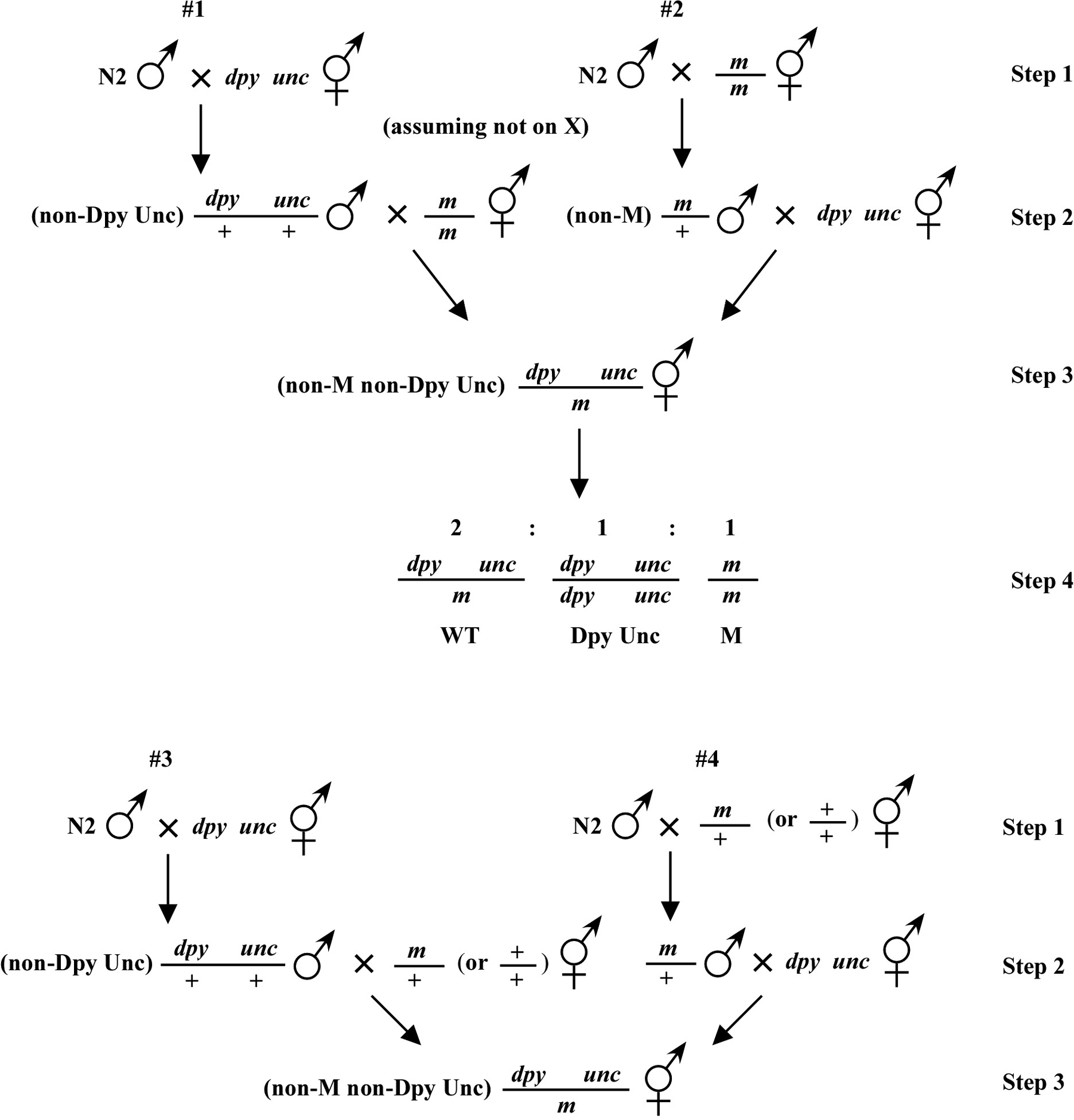
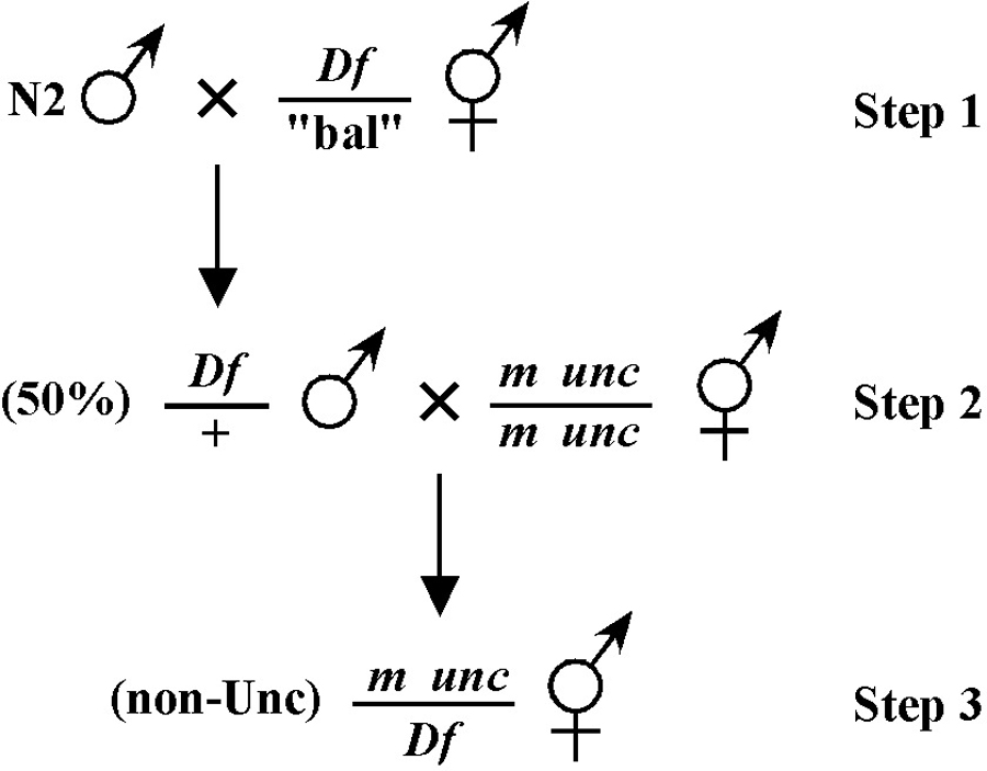
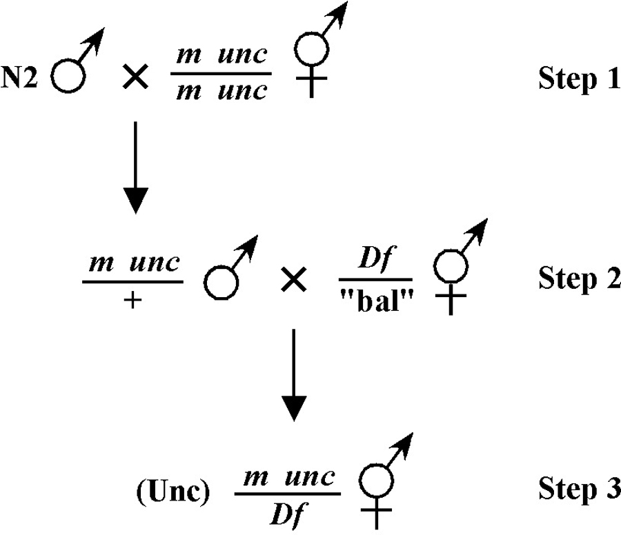
Beginning then with a stock of male animals, you will be able to set up matings between various mapping strains and your mutants. There are nearly always two ways to go here, as shown in Figure 3. You can either first cross N2 males into the mapping strain and then mate the male cross-progeny obtained into your mutant strain (schemes #1 and 3) or you can first cross N2 males to your mutants and then mate the male cross-progeny into your mapping strain (schemes #2 and 4). The basic goal in choosing one scheme over another is to maximize your efficiency by minimizing the number of cross-progeny that you will have to pick to recover sufficient numbers of animals of the desired genotype. Often genetic schemes will require that you pick “blindly” at certain steps, as you often won't be able to tell the difference between wild-type and heterozygous animals when working with mutations that are recessive. In addition, you may not be able to tell the difference between self- and cross-progeny when crossing into heterozygous strains. Clearly the best way to deduce the optimal scheme for your specific considerations will be by drawing it out both ways and then figuring out which method will be most efficient.
For the four schemes shown in Figure 3, the objective is simply to obtain dpy unc/m animals. If m animals are viable and easy to score, then either scheme #1 or #2 should suffice. The percentage of expected worms of genotype dpy unc/m at step 3 will be 50% for each, although positive assignment must wait until one can score the progeny at step 4. Also, in both cases, there will be no ambiguity associated with identifying cross-progeny produced by the matings in steps 1 and 2.
Consider the situation, however, where (m) is either lethal or sterile when homozygous. In this scenario, you will need to maintain m as a heterozygote (m/+), and all crosses into this strain will necessarily be made using m/+ animals. In this case, the two schemes (#3 and #4) would both theoretically result in 1/6 of the final progeny being of the desired genotype (calculate this yourself to ensure you understand). However, for scheme #3, you will be picking more blindly at step 3 than for scheme #4. This is because you won't be able to tell the difference between self- and cross-progeny at this step. Obviously, if the matings were to be 100% efficient, then this would not be an issue. But matings are never 100% efficient (often much less), and thus scheme #4 provides a clear advantage. Another potential reason to choose one scheme over another would be if the mutations were on the X chromosome. This is because the cross-progeny males generated at step 2 (either dpy unc/Ø or m/Ø) might be incapable of mating because a recessive allele on X will be expressed phenotypically in males.
As already stated, take the sledgehammer approach! Having too many males is not a problem. Having too few males is a big problem! Having too many cross-progeny is not a problem. Having too few cross-progeny can be a big problem! Get the idea? When setting up matings with strains that normally have low brood sizes such as DpyUncs adopt the more-the-merrier philosophy. For such matings you can put 15 males on a plate with an equal number of DpyUnc animals. Because you will be picking out non-DpyUnc cross-progeny, you need not worry much about the plates starving too quickly, as the wild-type cross-progeny will develop very rapidly as compared with the DpyUnc self-progeny.
For many matings it will be extremely important that you DO NOT inadvertently carry over any larvae or eggs from the male plate. Contamination of this type can quickly destroy a series of genetic crosses and if not detected can lead to erroneous conclusions. Better to first pick the males needed to a fresh plate, let them crawl around briefly, and then re-pick these “clean” males to the actual plates containing the hermaphrodites. Although this isn't always essential, it's best to just get into this habit and thus save yourself from trouble down the road.
Particularly when you are starting out, it is essential that you closely follow all your crosses to get a feeling for the normal progression and rate of the process. Otherwise, you could possibly mistake males used in a previous step for cross-progeny males. Also, if you inadvertently transferred a larvae or egg of the wrong genotype along with your males, you stand a chance of noticing and removing the offending animal before it creates any problems.
It is good practice to always choose virgin hermaphrodites when picking among your candidate cross-progeny animals. For some situations this may be more critical than others. However, the idea is that you usually want to see what the self-progeny of this virgin animal will segregate and don't want to complicate matters by having additional genotypes present. The safest way to do this is to pick cross-progeny hermaphrodites at the L4 stage. Whether or not an animal was a virgin can also be determined later by looking for males in the progeny. If present, the animal was obviously not a virgin, and you may want to discard such a plate in favor of one that displays the desired phenotypes but does not contain male animals.
When given a choice, pick cross-progeny animals from multiple plates where the mating has appeared to go well. For some situations, not every male will carry the chromosome that we desire them to contribute to the cross-progeny. When looking at cross-progeny on the plate, it is impossible to tell if they happen to be the spawn of one (lucky) male or many. However, the odds that we will pick cross-progeny that include the desired genotype end up in our favor if we pick from multiple plates. This is a further reason to set up multiple mating plates and to have a generous number of males on each mating plate. Things get chancy if we have to put all our eggs in one basket.
Do not carry over any contaminating larvae or eggs with your picked cross-progeny (also see above). If the plates from which you are picking are too crowded, simply remove the desired worms to either a clean portion of the same plate or to a new (intermediate) plate before re-picking.
Pick more candidate cross-progeny animals than you think are necessary. If you expect 25% of the cross-progeny animals to be of the correct genotype and you only need one or two, pick at least 20-40 animals anyway. Some may not be true cross-progeny. Some will crawl up the side of the plate and desiccate. Some may be damaged by picking. Odds may defy you. We have all had the experience of picking 50 animals, expecting to get at least 12 of the correct genotype, and actually getting only one! In this case, we are glad we picked 50! Picking a few more animals takes little time. Setting up the whole set of crosses again takes much time.
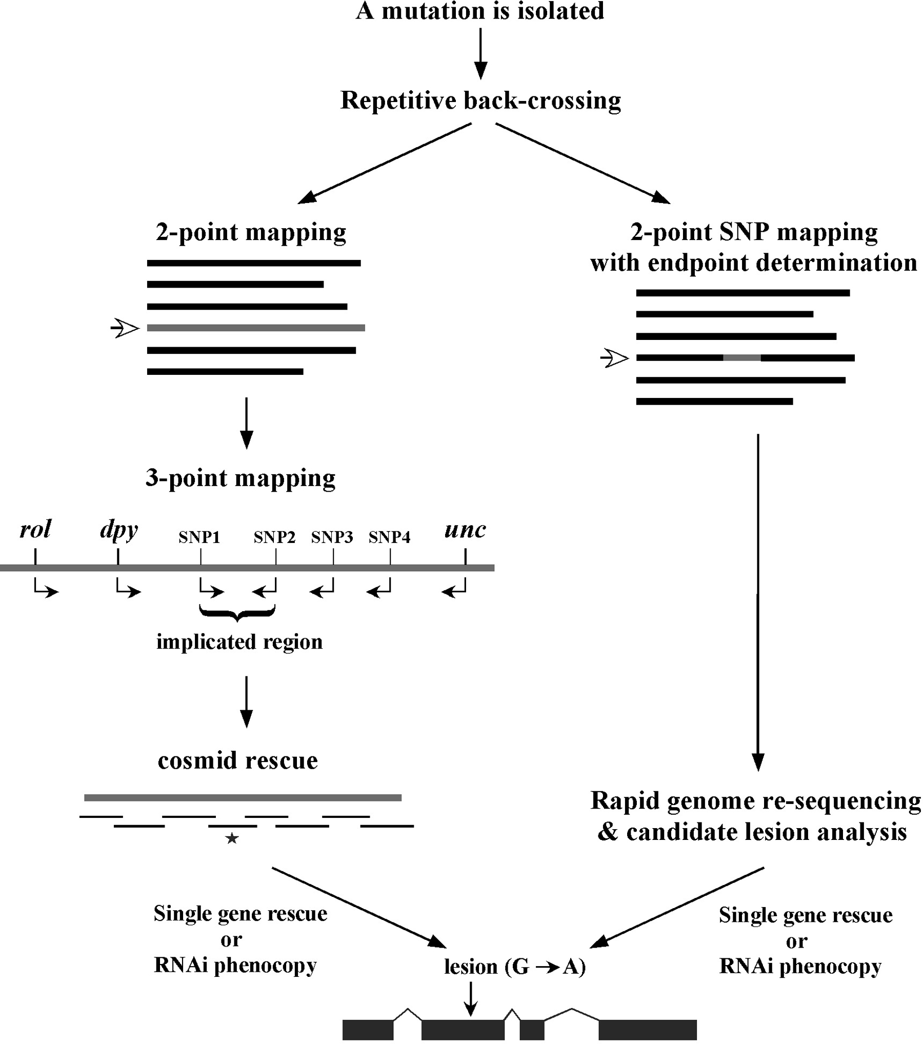
At this point, it is probably worth our time to delineate the progression of events that culminate in the cloning of one's mutation of interest. However, as alluded to in this section's introduction, standard methodolgies are a moving target. This is particulary the case in recent years, given the emergence of affordable and widely accessible genome re-sequencing methods. For this reason, two largely parallel paths are depicted in Figure 4. Note that both sequences initiate with the extensive back-crossing of the isolated mutation. This step is essential in order to remove the majority of unlinked background mutations accrued during random mutagenesis. Such background mutations can strongly affect the observed phenotypes and cloud interpretations. Although standard back-crossing practices may differ somehat between labs, a minimum of 5 independent backcrosses should be carried out prior to investing significant time on any mutant analyses.
In the classical approach, two-point mapping, using either standard genetic markers (Sections 2.2) or SNPs (Section 3.4), is used to place the mutation on one of the six chromosomes. In addition, two-point mapping also provides useful information regarding the approximate position of the mutation on the chromosome (Section 2.2.1). Three point mapping using genetic markers (Section 2.3) and SNPs (Section 3.6) is then employed to sequentially narrow down the region harboring the mutation. In some cases, SNP mapping allows the region of interest to be limited to just a handful of genes. Deficiency mapping (Section 4.1) is also useful for providing definitive terminal endpoints. Once the region of interest is sufficiently confined, researchers often attempt to rescue (revert) recessive mutations by creating transgenic strains carrying a wild-type version of the mutated gene. This is typically done by injecting regional cosmids or fosmids, which are low-copy bacterial vectors that contain ~20–40 kb inserts of wild-type C. elegans genomic DNA (see Transformation and microinjection). In addition to transgene rescue, it is also common to try and phenocopy loss-of-function phenotypes using RNAi methods (see Reverse genetics). Once a gene has been positively implicated (either by rescue, RNAi phenocopy, or both), the gene is sequenced to find the molecular lesion that is responsible for the defect.
While the above description lists the typical sequence of events using classical methods, historically various factors have lead to alterations in this strategy. For example, some regions of the genome were not amenable to cosmid or fosmid rescue because of lack of complete coverage. In those situations, RNAi might have been attempted before cosmid rescue, or regional candidate genes might have been sequenced in the absence of rescue or RNAi data. The bottom line is that every mapped mutation has undoubtedly had a slightly different history of identification. Some genes were relatively easy to clone while others were exceeding difficult, and it was impossible to predict a priori where any mutation might lie in this spectrum. In the end, the idea was to get from point A to point B in the most efficient manner possible. And while a positive wasn't guaranteed, diligence, care, and sweat were powerful weapons.
With the advent of next generation sequencing technologies, much of the exhaustive recombinant mapping and blind-rescue steps associated with classical approaches can now be circumvented in favor of directly identifying candidate lesions (Sarin et al., 2008). Following verification and prioritization of lesions based on their locations and the predicted consequence to protein structure and function, additional steps, such as RNAi-phenocopy and transgene rescue may be directly undertaken. Alternatively, if multiple alleles are available, the relevant gene is likely to pop out of the analysis as it will be mutated in independent strains. Furthermore, whole genome sequencing methods have been developed that circumvent the need for any classical and SNP mapping by making use of clustered mutations or SNPs acrued through the process of generating and back-crossing the isolated mutants (Doitsidou et al., 2010; Zuryn et al., 2010; Minevich et al., 2012).
Clearly, whole-gemone sequencing will play a huge role in the future of forward genetics in C. elegans, as well as many other systems. For one, sequencing methods will likely reduce the time spent on mutant gene identification by as much as an order of magitude. Furthermore, whole genome sequencing will largely eliminate existing inequities between different regions of the genome in terms of the ability to identify mutations. What's more, mutants that can only be assayed functionally in the context of complex genetic backgrounds, or where issues of low penetrance or subtle phenotypes render standard mapping approaches problematic, can now be tackled with relative ease.
With the advent of whole-genome sequencing appraoches, it is reasonable to ask whether or not the standard arsenal of genetic and SNP mapping methods are still relevant to the modern C. elegans researcher. I would contend that the answer in many cases is yes for the reasons listed below.
More than anything else, genetic mapping provides a litmus test for determining whether or not a given mutant is worth pursuing. In our own work, for example, we have encountered many situations where seemingly “good” mutants fail to behave in a normal Mendelian fashion when put to the rigors of mapping. The reasons for these occurances are often murky, but may in some cases be attributed to contributions from multiple loci or possibly even epigenetic phenomena. Regardless, the clear take home message is that such strains are probably not worth pursuing either by classical or modern sequencing methods. In general, if a mutant can be partially mapped, it is worth working on.
The mapping processes also faciliates the basic charatcerization of an allele's genetic properties. For example, is the allele dominant or recessive? Are there maternal or haploinsufficiency effects? Is the mutation a null or hypomorph? Mapping a mutation typically forces the researcher to contend with these questions and helps to provide clear answers.
Classical mapping with genetic markers also leads to the generation of useful reagents for use in further genetic and functional analyses. If the mutation is lethal or sterile, mapping will generate balanced strains for ease of propagation. Two and three-point mapping also allows the researcher to physically link their mutation to a visible marker. This is especially useful for mutations that lack overt phenotpyes and can be essential for carrying out complementation tests as well as tests for genetic suppression or enhancement.
Whole genome re-sequencing approaches will themselves be enormously aided by preliminary mapping studies. As an example, Sarin and colleagues (2008) mapped lys-12 to a 4-Mb region, thereby eliminating all but 5% of the total genes in the worm. In the absense of such mapping, many more of the detected candidate mutations would have required further experimental analysis. In fact, by confining the location of the mutation to a relatively small region, less total sequencing (genome coverage), may practically be required, thereby reducing incurred sequencing costs. Prior mapping is also likely to be critical in situations where only a single mutant allele exists or in cases where the mutation happens to affect a non-coding portion of the gene.
Classical mapping provides students with great training in genetics. Not that this is necessarily a sufficient reason to impose on others the continuation of a dead method—classical Sanger sequencing provided many scientists of my generation with great training in putting together fragile, slippery, transparent, radioactive jigsaw puzzles! Nevertheless, for undergraduate teaching labs, mapping mutations with visible markers drives home many of the key concepts and principles of Mendelian genetics.
Mapping with genetic markers is a highly reliable means for determining the approximate genetic/genomic locations of mutations of interest obtained through forward genetic screens. The materials conatined in this section describe much of what may now be considered the bedrock of “classical genetic mapping procedures”. That said, it should not be implied that these time-tested methods have now become totally irrelevant. To begin with, classical 2- and 3-point mapping provides an excellent platform for learning the theory behind other kinds of mapping methods, such as those involving single nucleotide polymorphisms (SNPs). Genetic mapping can also be used to confirm results obtained through other types of approaches and to generate a variety of highly useful reagents. For example, in cases where mutations of interest produce only subtle phenotypes, genetic mapping can generate linked strains, where one's mutation of interest (m) can be followed more easily based on the presence of a closely-linked cis visible maker (e.g., dpy m). Alternatively, lethal or sick mutations can be effectively balanced by placing visible makers in trans to the mutation (e.g., m/dpy), thereby greatly facilitating strain propagation and mutation retention. In addition, as described in the section on SNP mapping, the creation of singly (e.g., dpy m) or doubly (e.g., dpy m unc) marked mutant chromosomes is often essential for the detailed refinement of mutant genomic locations by 3-point SNP mapping.
Two-point mapping, wherein a mutation in the gene of interest is mapped against a marker mutation, is primarily used to assign mutations to individual chromosomes. It can also give at least a rough indication of distance between the mutation and the markers used. On the surface, the concept of two-point mapping to determine chromosomal linkage is relatively straightforward. It can, however, be the source of some confusion when it comes to processing the actual data based on phenotypic frequencies to accurately determine genetic distances. It is also worth noting that most researchers don't bother much with exhaustive two-point mapping anymore. Once we've assigned our mutation to a linkage group, it's generally off to the races with three-point and SNP mapping methods, or even whole genome sequencing, as these will almost always be necessary to clone our genes anyway. In fact, SNP mapping may in many cases be an excellent alternative to standard 2-point mapping using genetic mapping, and individual researchers will have to weigh the pros and cons of these methods for their particular situations. It is also worth noting that high-throughput methods for two-point mapping using SNPs (Section 3.4) have been used successfully by some groups and can provide a very precise map position for mutations. These methods may even (in some cases) allow for the molecular cloning of mutations in the absence of further three-point or SNP mapping (Wicks et al., 2001; Swan et al., 2002). Nevertheless, the vast majority of researchers still use some kind of tiered methodlogy in their cloning strategies for which two-point mapping (using SNP or genetic markers), is simply step one.
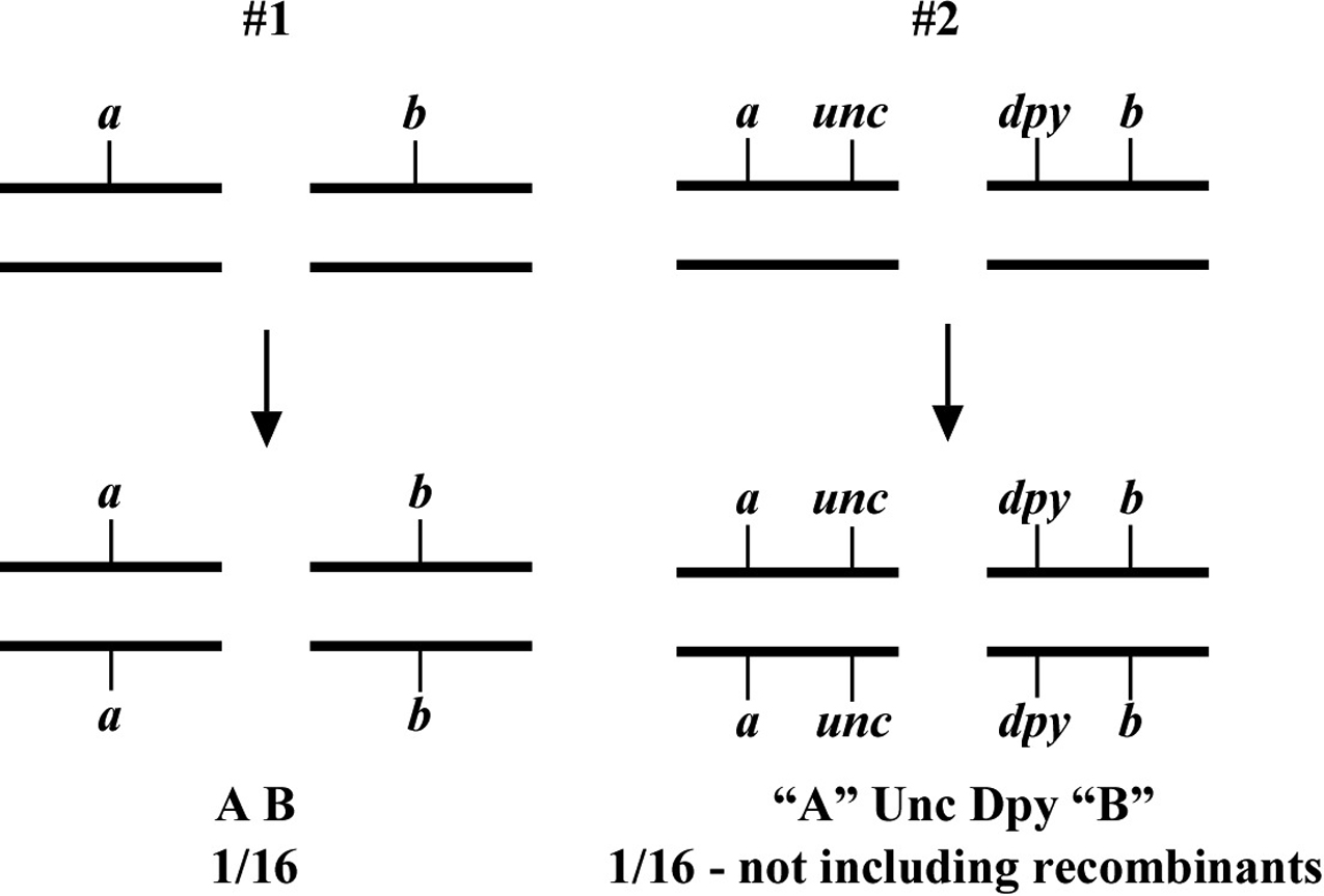
The two most basic outcomes for two-point mapping are shown in Figure 5. In outcome #1, the chromosomal position of the affected gene (mutation) happens to be on the same/homologous chromosome as the markers being tested. In this case, the mutation is actually flanked by the markers to produce a reasonably well-balanced strain. The genotypes of the progeny are indicated along with the ratios (or fractions) of their occurrences. Three genotypes are generated (m/a b, m/m, a b/a b) with three corresponding phenotypes (wild type, M, A B). In this situation we essentially never see the appearance of the triple mutant phenotype M A B, as this would require an exceedingly rare double-recombination event to take place. Furthermore, if we were to pick animals of phenotype M and examine their self-progeny, we would never see M A B animals. Likewise, A B animals will also fail to segregate M A B progeny. Finally, wild-type animals will always throw both M and A B along with wild-type animals. Seeing segregation patterns of this type tells us that m and a b reside on the same chromosome and also that m resides close to or in between the markers a and b. In the circumstance that the M phenotype is lethal, this may be a useful strain for maintaining m as a balanced heterozygote. Namely, by isolating wild-type segregants at each generation, we can propagate the mutation with relative ease. In addition, this strain can be used for three-point mapping (Section 2.3).
In contrast, the situation depicted in scheme #2 shows m and a b on distinct chromosomes. In the first generation, we therefore already expect to see 1/16 of the progeny displaying the triple-mutant phenotype M A B. In addition, if we specifically pick A B animals from this generation, 2/3 will throw M A B progeny. If necessary, draw out all the possible genotypes and corresponding phenotypes to convince yourself that these numbers are correct. Observing these kinds of segregation patterns indicates that the mutation and the markers are on different chromosomes. Another possibility is that the mutation resides on one of the ends of the chromosome (see below, Section 2.2.1). If necessary, these two possibilities can usually be resolved by scoring more animals. In general, basing linkage designation on a small number of data points (fewer than 20) should be avoided.
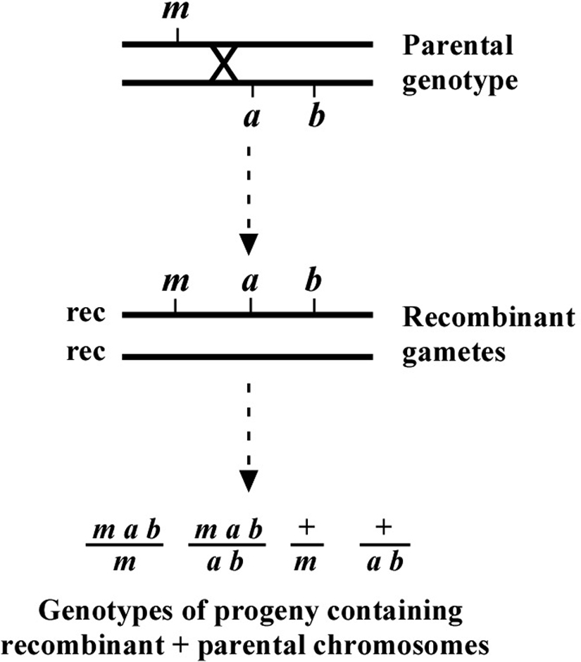
The genetic patterns described above are for the ideal situation where there is no ambiguity in the determination of chromosomal location. But what happens when the mutation lies to one side of the markers, perhaps at some distance? As shown in Figure 6, if the mutation lies to one side, a cross over may occur that will lead to the creation of the two recombinant chromosomes shown. One recombinant chromosome will now contain all three mutations in cis, whereas the other is completely wild type. Also shown are the genotypes occurring when such a recombinant chromosome is paired with one of the parental chromosomes. Now we have a situation where an animal of phenotype M or A B can throw M A B animals. In addition, a wild-type animal can now fail to throw both M and A B animals. In thinking about this, keep in mind that these “rare” recombinant chromosomes will usually, by chance, wind up paired with one of the non-recombinant parental chromosomes in a fertilized zygote. Of course, the farther the mutation is from the markers, the higher the proportion of recombinant chromosomes in the pool, and the greater the possibility that any two recombinant chromosomes may end up together in a zygote.
In these situations we must be careful not to hastily conclude that the presence of such genotypes automatically means that m and a b are on separate chromosomes. The question is more one of frequency. For example, if m and a b are 10.0 map units apart, this means that 10% of the gametes produced by the heterozygote will contain a chromosome that experienced a recombination event in this region. Worms are of course diploid, and progeny therefore have a chance to receive such a recombinant chromosome from either the sperm or the oocyte. Given this distance, the frequency with which progeny will inherit two non-recombinant (also called parental) chromosomes is 0.9 × 0.9 = 0.81 or 81%. The chance of progeny receiving two recombinant chromosomes will be quite small, in this case 0.1 × 0.1 = 1%. However, the frequency of progeny receiving one recombinant and one non-recombinant chromosome is 100 – 81 – 1 = 18%. A significant fraction!
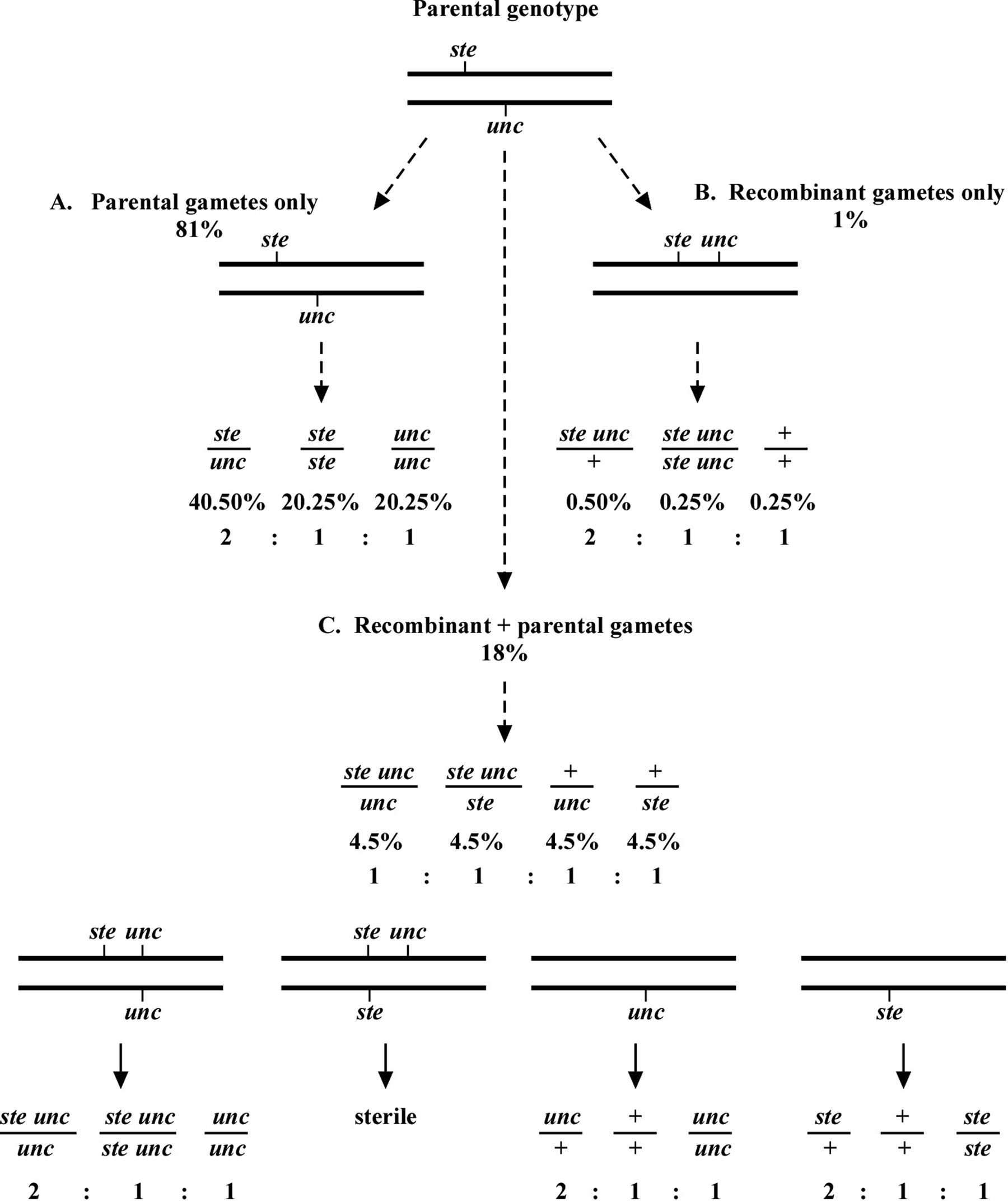
How then do we determine if a mutation is really on the same chromosome as the markers, and if so, what is the distance? This depends in part on how we are doing the mapping. Let us consider one specific example of mapping a sterile (ste) mutation relative to an unc mutation. In the example given in Figure 7, the ste and unc mutations are 10.0 map units apart. Again, this means that 90% of the gamete chromosomes will be of the parental type and 10% will be recombinant. As just stated, the chance of a progeny receiving two non-recombinant chromosomes will be 81% (Figure 7A), two recombinant chromosomes will be 1% (Figure 7B), and one recombinant plus one non-recombinant chromosome will be 18% (Figure 7C).
Of the recombinant chromosomes, one-half (5% of total chromosomes) will be ste unc and one-half (5%) will be wild type (+ +). Each recombinant chromosome has an equal chance of pairing with either of the two parental chromosomes. Therefore, for the animals that contain one recombinant and one non-recombinant chromosome, one-fourth will be ste unc/unc, one-fourth ste unc/ste, one-fourth +/unc, and one-fourth +/ste. These genotypes will therefore be present at a frequency of 0.25 × 0.18 = 0.045 or 4.5% each (Figure 7C).
Now consider mapping in the following way. From plates where the parent is ste/unc, we clone Unc progeny. We want to determine the frequency at which such Unc animals throw Ste Unc versus Unc only progeny. We therefore look for the presence of Ste Unc animals in the next generation. We know that there will be two genotypic possibilities for animals with an Unc phenotype, unc/unc, where both chromosomes are parental, and ste unc/unc, where we have one of each. The percentage of animals with the unc/unc genotype is 0.81 × 0.25 = 0.2025 (20.25%), as 81% will have only parental chromosomes and of these, one-fourth will receive two unc chromosomes. The percentage with a ste unc/unc genotype will be 0.18 × 0.25 = 0.045 (4.5%), as 18% of progeny will have one recombinant and one parental chromosome and there is a 25% chance of receiving both the ste unc and the unc chromosome (0.5 × 0.5 = 0.25). The overall percentage of animals with an Unc phenotype will therefore be 4.5 + 20.25 = 24.75%. Finally, the percentage of Unc animals with a ste unc/unc genotype will be 4.5/24.75 = 18.2%.
The above determination tells us that if our mutation and marker(s) are 10.0 map units apart, we should expect to see about 18% of the cloned Uncs throwing Ste Unc progeny. Similar calculations can be carried out for various genetic distances. To facilitate these determinations, the formula (1-p)(1-p)/4 (where p is the map distance expressed as a fraction, e.g., 10 map units = 0.1) can be used to calculate the predicted fraction of unc/unc animals, whereas the fraction of ste unc/unc animals can be calculated using the formula 2p(1-p)/4. The total sum of these two products will give the fraction of all Unc animals, and the relative percentage of recombinant genotypes (ste unc/unc) can be obtained by dividing the fraction of ste unc/unc animals from the total sum. For example, if the marker and mutation are 1.0 map unit apart, we will see Ste Unc animals appearing from ~ 2% of the cloned Uncs. At 5.0 map units apart, it will be ~ 9.5%; at 25.0 map units, ~40%. The general rule is that when mapping by this strategy, the frequency of animals containing the recombinant chromosome will be about double that of the map distance between the marker and the mutation. As the distance between the mutation and marker increases, this frequency decreases.
Interestingly, by the time we get to 50.0 map units, 67% or 2/3 of Unc animals will throw Ste Unc progeny. This latter number should sound familiar; it's the same percentage you would get if the ste and unc mutations were on separate chromosomes. In fact, at 50.0 map units or greater, two mutations will appear to be unlinked. This usually is not an issue because we tend to carry out two-point mapping with markers at the chromosome center, guaranteeing distances no greater than about 25.0 map units.
There are often multiple ways to carry out two-point mapping using the same set of markers. For example, in the previously described cross we could have picked wild-type rather than Unc animals and looked for the absence of either Unc or Ste animals in their progeny, signifying a + + or wild-type recombinant chromosome. If the marker and mutation are 10.0 map units apart, we will predict to have 0.81 × 0.5 = 40.5% of animals with an unc/ste genotype. We will also have 0.18 × 0.5 = 9% of animals with either an unc/+ or ste/+ genotype (4.5% each). Thus we predict that 9.0/49.5 = 18.2% of the wild-type animals we pick will fail to segregate either Unc or Ste progeny. These numbers are identical to those previously calculated for picking Unc progeny and looking for Ste Unc in the next generation.
Consider this final case however. Imagine you are trying to map an embryonic lethal mutation (emb) relative to a known unc. The easiest way to do this would be to pick wild-type animals from an emb/unc parent and then look for the absence of Unc animals in the progeny (embryonic lethals are usually difficult to score directly by their plate phenotype). If the unc and emb are on the same chromosome and close, very few phenotypically wild-type animals will fail to throw Unc (as well as Emb) progeny. To calculate the map distance, however, we must realize that using our methods, unc/+ animals will not be among those counted as “recombinants” (those wild-type animals that fail to throw Uncs). Thus, if the distance between the unc and emb is 10.0 map units, we predict to have 0.81 × 0.5 = 40.5% animals of genotype emb/unc. We will also have 0.18 × 0.25 = 4.5% of animals with an emb/+ genotype and 4.5% with an unc/+ genotype. Therefore, when picking among the phenotypically wild-type animals, the frequency of emb/+ animals will be 4.5/(40.5+4.5+4.5) = 9.1% (and not 18.2%) of the total. Being aware of these factors and, as always, drawing out the cross carefully will prevent interpretive errors. For a discussion of additional two-point mapping strategies as well as potentially useful formulas for correlating map distances with phenotypes, see Hodgkin (1999).
A question of strategy—to map all chromosomes at once or to do so sequentially? This may depend on several factors such as time constraints and competitive pressures. Everything being equal, mapping sequentially is the most efficient allocation of time because once one has positively identified a chromosomal location, one need not check all the other chromosomes. In practice though, we often want to map our mutants as quickly as possible and will test multiple chromosomes at once. In addition, the presence of clear negative data can strengthen conclusions when the mutation lies at some distance from the markers. Along these lines, it is worth noting that a number of strains containing markers for multiple chromosomes have been generated for the express purpose of enhancing mapping efficiency. For example, strain MT464 contains the markers unc-5, dpy-11, and lon-2, thereby permitting the simultaneous mapping of chromosomes IV, V, and X, respectively. Also, in considering the X chromosome, recall that recessive mutations on X will be generally express the mutant phenotype specifically in cross progeny males that are X/Ø. This situation can be easily distinguised from standard dominant mutations, in which the phenotype would be expressed in both cross-progeny males and hermaphrodites.
It is also worth pointing out that an observant experimentalist can often get a good sneak peak at what the three-point data will ultimately confirm during the two-point mapping process! In fact, this is another good reason to carry out two-point mapping using adjacent markers. To reiterate, we already know that if the mutation (m) happens to be on the same chromosome as the markers a and b, then the large majority of M animals coming from the heterozygous parent (m/a b) will fail to throw A B progeny. Because of recombination, however, you may observe a small percentage of M animals throwing either M A, M B, or M A B animals. For example, if you happened to observe three plates (out of 25) with M A B animals and one plate with M A animals, that would suggest that m lies to right of b and is at some distance from the markers. In contrast, if you were to only observe several plates with M A animals, m would be likely to lie to the right of b but close to the markers (or perhaps between them and just to the left of b). If M A B animals are never observed but there are a small percentage of M A and M B animals, then m must lie between the markers. If this reasoning is not yet clear, read over the three-point mapping discussion below and then draw this out to confirm the predictions. This bonus gift of two-point mapping can be a real time saver.
Once you have assigned your mutation to a chromosome, the next step using the classical genetic approach is three-point mapping. Three-point mapping has traditionally been the backbone of worm genetics and has historically almost always an obligatory step in the process of cloning our mutants. Even SNP mapping (discussed in Section 3), is really just a high-tech variation of classical three-point mapping and is usually preceded by three-point mapping with genetic markers. The basic idea is that we cross our mutation (m) into a strain with two linked morphological markers (a and b) that are on the same chromosome as m, to generate the m/a b heterozygote. We then isolate and follow two classes of recombinant progeny; those that display the A phenotype only (A non-B recombinants) and those that display only the B phenotype only (B non-A recombinants). By seeing which of these two classes produce the mutant phenotype (M) and by scoring the percentages for each, we can determine whether our mutation lies to the left, to the right, or between our set of markers. In the case where the mutation lies in between, we may then determine the approximate distance from each marker.
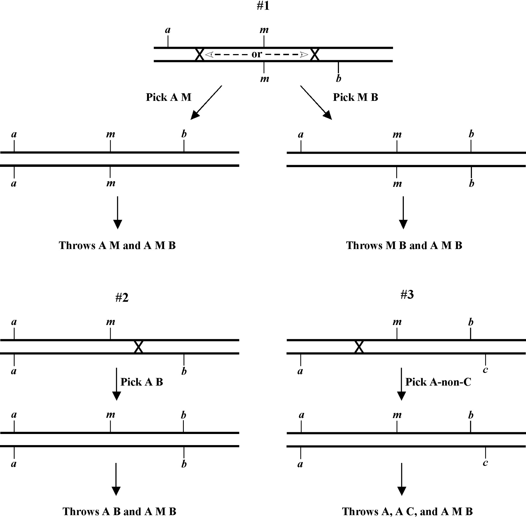
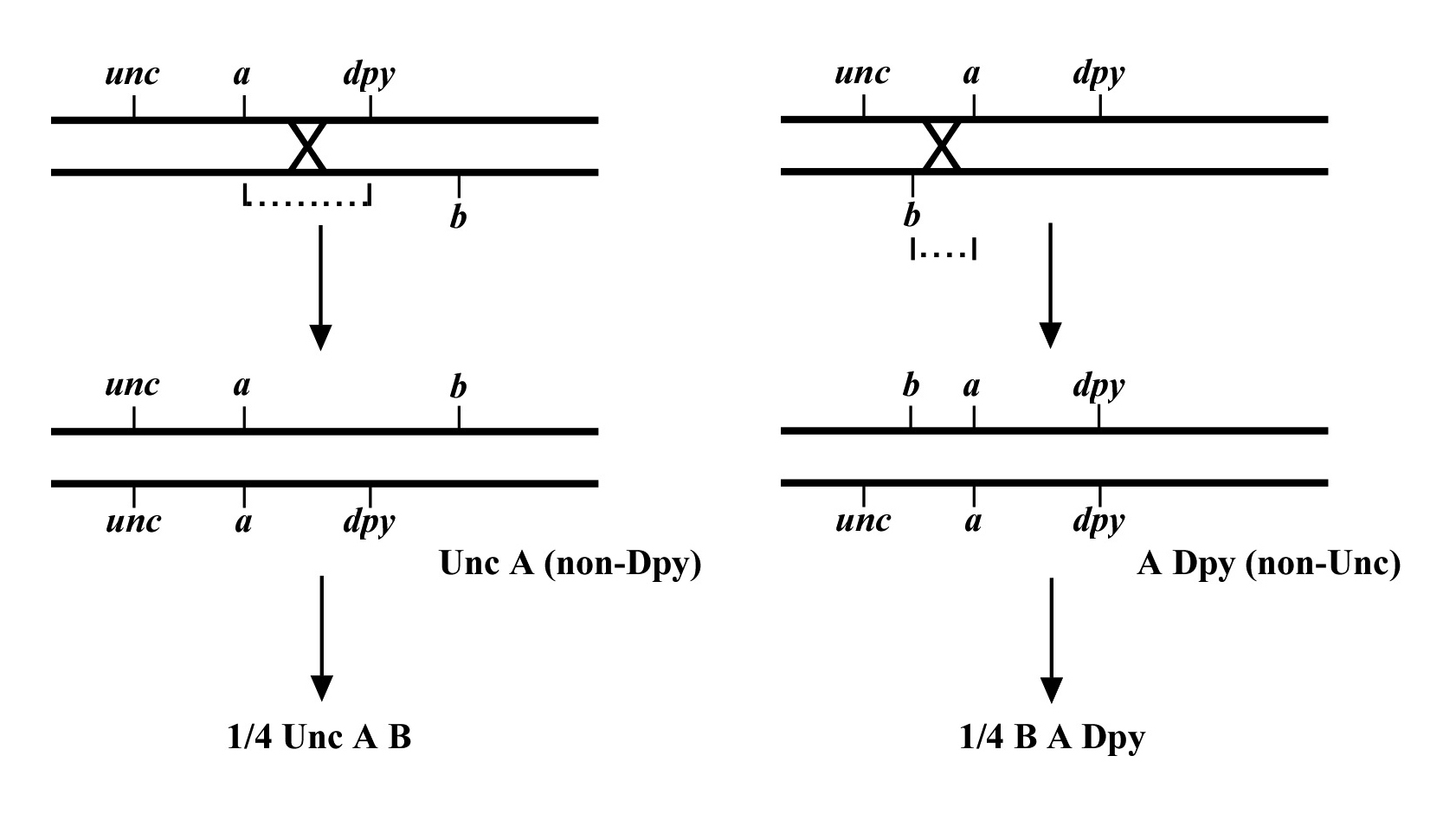
Figure 8 depicts the outcome of a recombination between markers a and b when m lies either to the left or right of the markers. When m lies to the left, essentially all B non-A recombinant animals will throw ¼ B M progeny (as well as B and A B), whereas A non-B recombinant animals will throw only A and A B progeny. When we see this kind of pattern, we can conclude that m lies to the left of a or perhaps to the right of a but very close. The reason for this is that if m were very close to a but between a and b, the frequency of generating the a m recombinant chromosome would be very low (also see below). Thus although m is most likely to the left of a, we often have this caveat. Greater numbers of recombinants can help to diminish this possibility, if not rule it out completely. The situation for m lying to the right is simply the reverse.
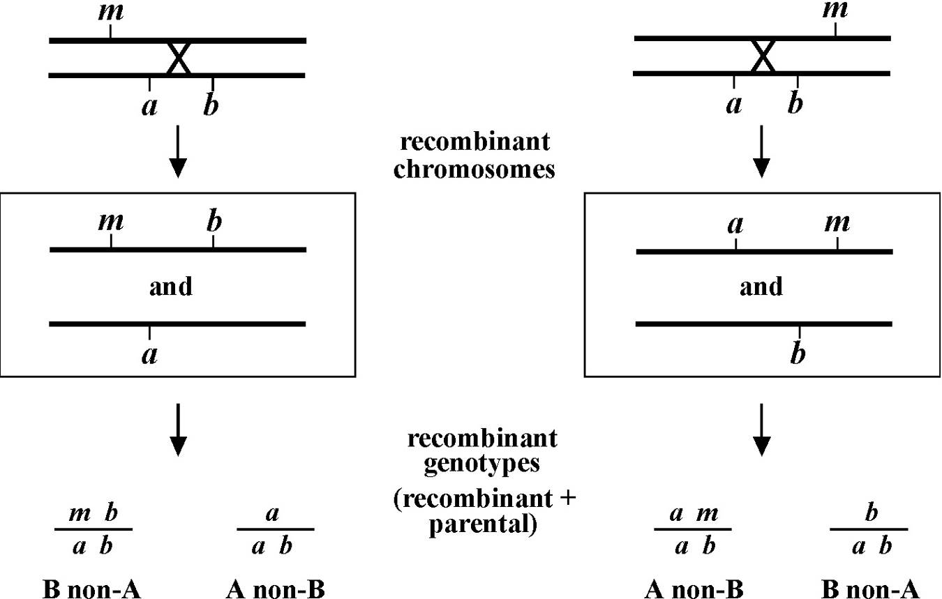
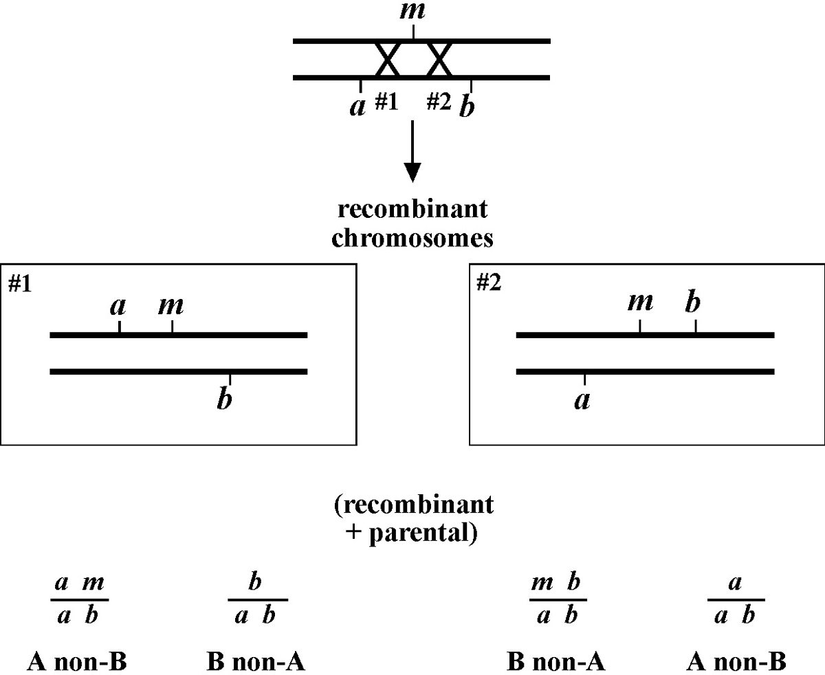
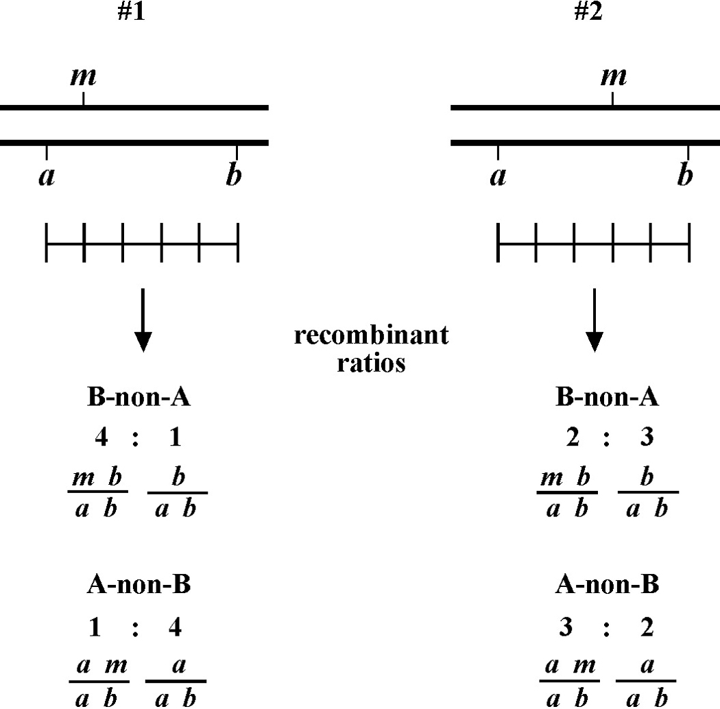
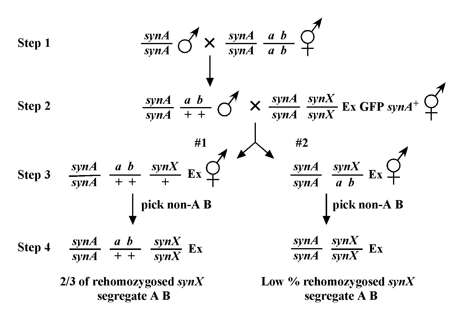
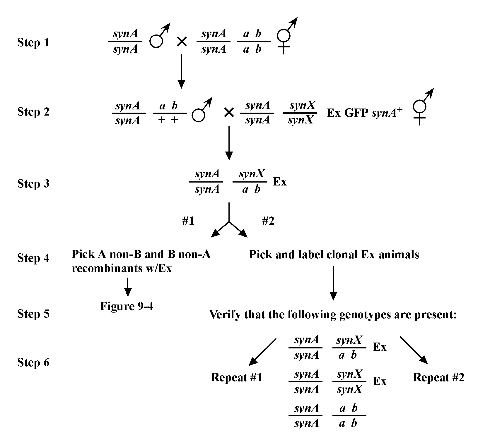
The mapping described above, though useful, only tells us that m is likely to be left or right of our given markers. It doesn't provide any information about how far from these markers m might reside. To determine this we need to use markers that flank m, as shown in Figure 9. Here we see that depending on the site of the cross over, A non-B recombinant animals can in some cases acquire m (#1) and in other cases not (#2). The same is true for B non-A animals. In three-point mapping, we seek to determine the ratio of recombinant animals that pick up the mutation versus those that do not. This ratio provides us with a direct genetic position for the mutation as illustrated in Figure 10.
Here markers a and b are in cis and are located 5.0 map units apart, whereas our mutation, m, is in trans to a and b. In the situation on the left, were we to pick B non-A recombinant animals, four-fifths or 80% would be expected to carry m in cis to b. A non-B recombinants, on the other hand, would acquire m only one-fifth or 20% of the time. On the right, B non-A animals will acquire m only 40% of the time, whereas A non-B animals will acquire it 60% of the time. Obviously, when picking recombinants from both sides, the numbers should converge on a single location, i.e., the frequencies should add up to 100%. These numbers can be used to specifically assign a genetic location. For example, in the left diagram, if a were at genetic position 0.0 on the chromosome and b at 5.0, having 20% of A non-B recombinants acquire m would lead to a map position assignment of 1.0. Obviously, the greater the number of recombinants scored, the greater the certainty of the assignment.
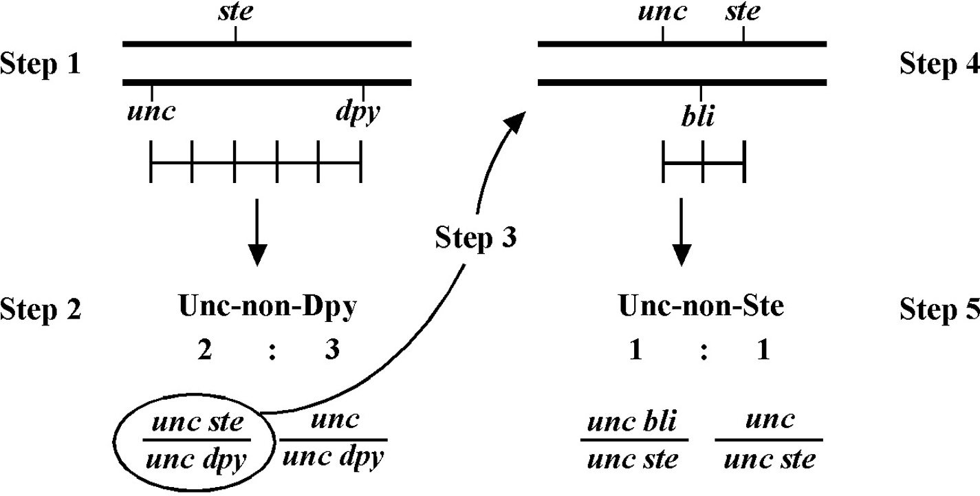
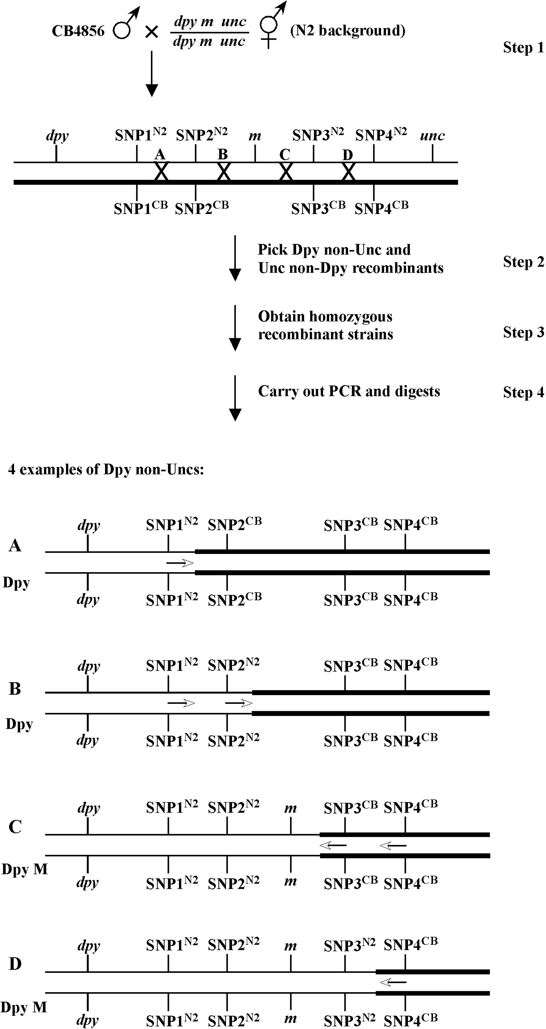
Always save recombinants; they often prove very useful for subsequent mapping, not to mention genetic studies where having a linked marker may prove indispensable. Figure 11 shows an example of how to use the recombinant chromosome for further mapping (also see Section 4, Mapping with deficiencies and duplications). Imagine we are mapping a ste mutation and have placed it between unc and dpy markers that are separated by 5.0 map units (step 1). The ratios place the ste mutation closer to the unc marker (10 out of 25 Unc non-Dpy recombinant animals threw Unc Ste progeny; step 2). We save theunc ste/unc dpy strain and cross it to a strain that is homozygous for a bli mutation (step 3). We obtain the strain shown in step 4 and then screen for Unc non-Ste animals (step 5). In this case, 50% of the Unc non-Ste recombinants acquired the bli mutation, placing ste and unc mutations at an equal distance (but on opposite sides) from bli.
In this way, we continue to refine the map position of our mutation. Usually the data from different mapping schemes will tend to agree, although not always. This may be due to a number of factors. In general, the farther apart the markers are, the less precise the mapping tends to be. Thus we put more weight on data acquired using nearby markers than those that are at some distance. In addition, it is highly advisable to map using markers that have already been cloned. This provides a precise chromosomal location and allows one to compare directly the genetic and physical maps. If you have no choice but to use a non-cloned mutant for mapping purposes, check Wormbase or journal articles for information regarding how this gene was mapped to its present location.
What happens if you initially map your mutation to the wrong chromosome and then try to carry out three-point mapping? Essentially, your mutation segregates independently of the recombinant chromosome and will be picked up two-thirds of the time. Thus, if for example, 67% of your Dpy non-Unc and Unc non-Dpy animals throw your mutation, you may want to consider revisiting your two-point mapping data.
Another thing to be aware of is the possibility of either multiple crossovers events or double recombinants. Multiple crossovers occur when two or more recombination events have taken place on a single chromosome during meiosis. Although such events are purportedly extremely rare, they can happen, and the larger the number of recombinants scored, the greater the possibility that this could be an issue. For this reason, it is generally wise to stick to markers that are approximately 5.0 map units apart when doing three-point mapping. In any case, always be aware of this possibility and refine your interpretations if necessary. Double recombinants simply refer to worms that contain two recombinant (non-parental) chromosomes. These are quite obvious to spot, as they will only throw recombinant progeny. For example, if you pick a Dpy non-Unc and it throws only Dpys (no Dpy Uncs), then both chromosomes must have been recombinant. You will want to toss such strains as they could contain a mixture of dpy and dpy m chromosomes, which would unduly complicate things. As with multiple cross over events, the chance for double recombinants increases as the distance increases between the markers.
At the most basic level, two things should be anticipated in advance of picking recombinants for mapping: 1) the expected frequency of recombinants; and 2) the plate phenotype(s) of the recombinant animals. The first concern is relatively easy to calculate. Because you should know the distance between the two genetic markers, the frequency of recombination events between these markers can be directly determined. For example, if two markers (a and b) are 2.0 map units apart, then a crossover event will occur between a and b in 2% of the chromatid pairs (4% of the tetrads) leading to 1% of the gametes containing an a-only chromosome and 1% containing a b-only chromosome. Because hermaphrodite worms are diploid for all chromosomes, this effectively doubles the chance of acquiring a recombinant chromosome in the progeny, as it can come from either the sperm or the oocyte. To detect the recombinant, however, it must be over the ‘correct’ parental chromosome (a b), which will occur only 50% of the time. The end result is that if one is looking specifically for A non-B recombinants, and a and b are 2.0 map units apart, then an animal with an A non-B phenotype will occur on average about 1% of the time. Likewise, B non-A animals will occur 1% of the time. Obviously, if the mapping allows picking of either A non-B or B non-A non-recombinants, this will effectively double the total number of recombinant animals that can be obtained from a given number of plates.
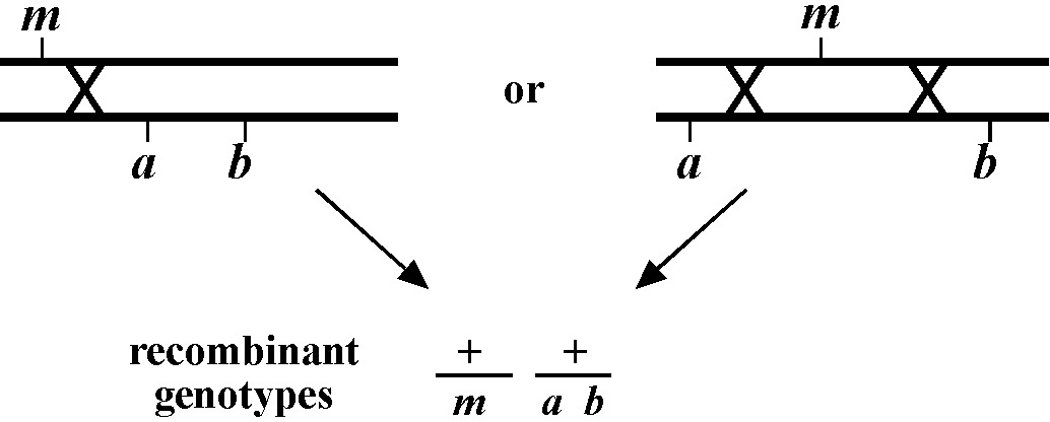
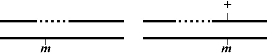
The next step is to recognize and pick the recombinant animals. But first it is important before picking from any plate to ask the question: Do the animals on this plate display the expected phenotypes? In effect, you are thereby asking: Did the parental animal have the correct genotype? This is exceedingly important to determine before picking any recombinants. The reason is that recombination events may have occurred in the previous generation such that the cloned parental animal may not have had the correct genotype. For example, you may have picked phenotypically wild-type animals from a plate where the parental animal was of genotype m/a b. Given that self-progeny with the genotype m/a b will be wild type, you might imagine that you are safe in assuming that all wild-type progeny will therefore have genotype m/a b. But imagine the following two scenarios depicted in Figure 12. In the scenario on the left, m lies to one side of the markers a and b. A recombination event between the markers and m can result in the creation of a wild-type chromosome (+) as well as a triple mutant chromosome (not shown). Therefore, when the recombinant + chromosome is paired with one of the parental chromosomes, phenotypically wild-type animals would be generated with the genotype m/+ or +/a b (and not the expected m/a b). Likewise, animals of m/a genotypes (though probably not m/b) could arise following a single recombination event between a and b. For the case on the right, a double recombination event would have to occur to generate a wild-type chromosome, and this will admittedly be very rare. A single recombination event, however, could result in either m/a or m/b animals, which will also appear phenotypically wild type (also see below).
Clearly, one does not want to pick recombinants from plates where the parental animal had the incorrect genotype. This will wreak havoc on one's mapping and lead to incorrect conclusions. The solution is simple: Make sure the phenotypes observed on the plate correspond to the correct parental genotype. For example, if the parental animal has the expected genotype m/a b, then one should see wild-type animals (m/a b), M animals (m/m), and A B animals (a b/a b). In addition, it should be possible to find occasional recombinant animals (A non-B and B non-A), which is exactly what you are looking for. Although simple in practice, fundamental errors by novice mappers are not uncommon. For example, some Dpy mutants may appear partially Unc, thus, loss of the unc mutation could initially go unnoticed. Other markers such as let and egl may require even greater care to maintain. In the end, strict diligence is the only weapon against such mistakes. Bottom line: Do whatever you consider necessary to ensure that recombinants are obtained only from plates with the correct parental genotype.
Recognizing the recombinants that you want may not be trivial! Or it may be, depending on the nature of the mutant phenotypes and your level of experience. For example, you acquire a dpy unc strain for mapping purposes and the double-mutant animals indeed look both Dpy and Unc, but what will the Dpy non-Unc or the Unc non-Dpy recombinant animals actually look like? Often one does not have either the dpy or unc mutation alone for comparison. In the absence of having the single-mutant strains available, the best approach is to read up on the descriptions of the single mutant phenotypes, ask experienced members of your lab for advice, and keep handy the double mutant strain for comparison to any potential recombinants. Once you have isolated a few true recombinants, finding new ones will suddenly get much easier.
How many recombinants should one pick from any given plate? This may depend on several factors. As a rule, be very cautious of plates where you seem to have hit a “gold mine”! (“Wow, I can get all 20 recombinants off of one plate!” NOT.) The simplest explanation when encountering such a plate is that a recombination event must have occurred in the previous generation to affect the parent. This is precisely the situation that was described above. Looking at such plates it will probably be clear that the parent animal did not have the correct genotype. In this case, it is permissible to pick a single recombinant animal, as this does represent one legitimate recombination event. However, even in cases where most animals correspond to the non-recombinant phenotypes (indicating that a parental recombination event did not occur), it is still advisable to pick only 2 or 3 recombinant progeny from any one plate. The (perhaps overly paranoid) worry is that a rare mitotic recombination event could have occurred in the germline to generate a clone of identical recombinant sperm or oocytes.
Often when looking for recombinants to pick, one will examine the same set of plates for several days in a row. It is a common experience that recombinants that are ‘invisible’ one day will jump out at you the next. Certainly for some types of mutants such as ste or egl, the recombinant phenotype may only be obvious once animals are well into adulthood. When scanning the same set of plates over several days, keep whatever notes necessary to ensure that you don't keep picking your recombinants off the same plate without knowing it. Proper note taking and labeling of plates will prevent this from happening.
What happens if you accidentally pick a non-recombinant animal by mistake? No problem, as it should be quite obvious when looking at progeny in the next generation that a recombinant was not picked. For example, if you attempted to pick a Dpy non-Unc animal and notice several days later that the “recombinant” worm has failed to throw appreciable numbers of Dpy non-Unc animals, or is perhaps throwing phenotypically wild-type animals, obviously the parental animal was not a true recombinant. Chuck the plate and move on. It is better to pick some false recombinants (and eliminate them later) than to miss picking any true recombinants.
A note of caution: Make sure that when picking recombinants, you do not carry over contaminating eggs or larvae! This is surprisingly easy to do and will usually ruin your ability to score that particular recombinant since the plate will be contaminated with animals of non-recombinant phenotypes. If the plate is crowded, move the recombinant animals to a less populated region of the plate in order to clean the recombinant animal of larvae or eggs that may have stuck to its side. Sometimes it may even be necessary to transfer the recombinant to a ‘clean-up’ plate before cloning to its own plate. As a second line of defense, always watch the recombinant animal after transferring it to its own plate and destroy any contaminating eggs or larvae that may come off. Such procedures become second nature very quickly.
The presence of certain phenotypes may prevent that accurate scoring of other phenotypes. For example, the Bli (blister) phenotype is often masked (suppressed) by dpy and rol mutations; unc mutations may mask the Rol phenotype; dpy mutations will usually mask a Lon (long) phenotype; certain dpy and unc mutations may sometimes appear Egl, etc. Obviously, there may be a lot to consider, and going into the mapping well informed is essential. Surprisingly, one can sometimes map with mutations that would seem unlikely. For example, it may be possible to identify certain UncX non-UncY mutants, depending on the nature of the two Unc phenotypes.
It is highly recommended that you render your phenotypic judgments on animals that have been propagated on clean plates containing sufficient OP50. Many bacterial contaminants can actually prevent the accurate scoring of Unc and Ste phenotypes in genetic crosses. In addition, starved plates can lead to erroneous conclusions regarding sterility, brood sizes, Egl, and other phenotypes. If in doubt, you can always bleach your strains and reassess phenotypes later from clean plates. Better yet, make sure that your plates and strains are clean before initiating the mapping process.
Clearly, the most efficient type of three-point mapping would allow for picking of recombinants from “both” directions. For example, one can pick Unc non-Dpy and Dpy non-Unc recombinant animals from a strain with a dpy unc chromosome. The benefit of this setup is that it effectively doubles the number of recombinants obtained from a given number of plates, and provides independent mapping information from both types of recombinants (which will hopefully correspond!). It is not uncommon, however, that the markers will dictate that only one of two possible recombinants is picked. For example, when looking for recombinants between unc and let (lethal) mutations, it will only be possible to identify and pick Unc non-Lets for obvious reasons. The same thing occurs when using markers that confer a sterile phenotype, in situations where one of the markers masks the phenotype of the other (e.g., Rol non-Uncs versus Unc non-Rols), or where penetrance is an issue (see above).
Finally, as with all genetics, it is wise to pick more worms than is anticipated to be necessary. The rate-limiting step for all genetics is growth of the animals, and not the time required to transfer a few more worms to plates. Still, there is a limit to how much information can be gleaned from any one cross, and good researchers are always efficient in the use of their time.
When is one done with three-point mapping? Before the advent of SNP mapping and whole genome sequencing, the common strategy was to play out all of one's cards. Namely, you would use every available genetic marker or chromosomal rearrangement to minimize the size of the genetic region known (or likely) to contain your mutation. Once this was done, cosmid injections to obtain rescue could begin. Of course, the paucity of markers in many regions often meant that many cosmids would have to be injected (not a trivial task). Even worse, for many regions, complete cosmid or fosmid coverage was very incomplete. As described in Section 3, the situation became considerably less dire with the advent of SNP mapping in the late 1990's, and although standard three-point mapping was still useful to some extent, it was not done so exhaustively. Thus to answer the initial query—one often ceased with three-point mapping when the mutation had been placed within a 1- to 5-map unit region bounded by two solid genetic markers which correspond to known locations the physical map (i.e., the markers have been cloned). Having said that, if the region was rich with genetic markers, there was often no particular reason to stop genetic mapping all together. In some circumstances, it was still be the most efficient means by which to narrow down the region of interest to a workable size for injections or candidate cloning and, at the very least, the process itself generated additional useful reagents.
Regardless of the stage at which genetic mapping was concluded, it was common practice to use mapping data to find ground zero on the physical map; that is, the stretch of DNA where your mutation is predicted to reside. The old-fashioned way to do this was to construct a complete graphic of the physical map for the region, a process that required some actual cutting and pasting of a printout of the map. One then took actual physical measurements of the distances between the markers used (e.g., 135 mm) and, based on the obtained mapping data, found the point on the chromosome that has been implicated. More recently, one can avoid the graphic map entirely by calculating the predicted site of the mutation based on the numerical chromosomal locations of the markers used (e.g., 9,279,450). This is quite straightforward and eliminates potential errors associated with any graphic representation. Detailed information for this purpose can be found on Wormbase.
It should be pointed out that while it may have been satisfying to point to a single base pair on the chromosome as being the most likely site of one's mutation, this prediction was only as good as the mapping data. Furthermore, regional variations in recombination frequency along the chromosome can lead to significant discrepancies between the actual locations of genes and those predicted using these methods. Still, this method was useful for predicting which SNPs would be most appropriate for testing first, or if the region was small enough, to compile a list of likely rescuing cosmids or fosmids in order to prioritize the order of injections.
Mapping with single nucleotide polymorphisms (SNPs) is a powerful complement (and in some cases outright alternative) to mapping with genetic markers (Section 2). With SNPs, basically all mutations became theoretically mappable using standard lab procedures, something that wasn't true in the past. Moreover, SNP mapping could be routinely used to narrow down the known physical location of mutations to regions smaller than a single cosmid (~30,000 bp; ~6-7 genes). With genetic mapping, even in the best of circumstances, the implicated regions usually spanned 6-10 complete cosmids or more. In fact, SNP mapping can theoretically be used to narrow down the implicated region to a single gene, although this level of mapping is usually unnecessary and can become inordinately time consuming.
Although several approaches for mapping using polymorphisms have been described, we will focus here on the use the Hawaiian C. elegans isolate, CB4856 (Jakubowski and Kornfeld, 1999:; Koch et al., 2000:; Wicks et al., 2001:; Swan et al., 2002:). Geographical separation and evolutionary drift have led to a sizeable number of genetic differences (DNA polymorphisms) between the Hawaiian (CB4856) and English (N2) C. elegans isolates. In fact, differences in the genomic sequences of CB4856 and N2 occur on average every 1,000 base pairs. The majority of these changes occur in non-coding or intergenic regions and probably have no functional consequence. Some polymorphisms, however, clearly affect protein activity or gene expression, as N2 and CB4856 differ notably in a number of respects including their mating behaviors and relative sensitivities to RNAi (Tijsternman et al., 2002:).
The term SNP is a bit of a misnomer. Although many of the sequence variations between N2 and CB4856 are indeed single-nucleotide changes (for example from an A to a G), small deletions or insertions are also very common. What is experimentally most relevant, however, is whether or not these polymorphisms affect the recognition site for an endonuclease. SNPs that result in restriction-fragment length polymorphisms (RFLPs; also called snip SNPs) are easier to work with, as digestion by enzymes is much more rapid and inexpensive than sending off samples for sequencing. Also, it generally doesn't matter whether it's the N2 or CB4856 DNA that is cleavable (however, also see Section 3.4), just so long as the digestion patterns of the two isolates are clearly distinguishable.
Over the past 15 years various internet-accessible C. elegans SNP databases have come and gone. In fact, some of the better ones, with respect to the user interface, no longer exist. One consistent way to access SNPs is directly has been through WormBase. To view SNPs on WormBase simply go to your region of interest using the WormBase genome browser (GBrowse under the Tools menu) and select a reasonably-sized genomic region for viewing (e.g., 10 kbp). If SNPs are not visible, check the “Polymorphisms” box under the “Select Tracks” option and click “Back to Browser”. This will display the predicted SNPs in the region as diamonds. Other glyphs indicate deletions (boxes) and insertions (triangles). Yellow diamonds indicate SNPs identified in CB4856 (Hawaii), blue SNPs identified in CB4858 (Pasadena), and white SNPs from all other sources. Clicking on the diamonds or adjacent text brings you to a new page where you have the option of viewing an expanded region (500 bp) surrounding the SNP. (Hint: it is easier to perform this click option when the selected size of the region is 5 kbp.) Note that it is necessary to cut and paste these sequences into a restriction enzyme digestion program to determine whether or not the predicted SNPs lead to RFLPs, which are much more useful than non-RFLP SNPs that can only be identified by sequencing. Additionally, the reliability of the unconfirmed class of SNPs on WormBase is currently unclear, although most are likely to be valid. In any case, empirical testing of any SNP to be used for mapping is essential before examining experimental recombinants.
An assessment of any SNP requires that the chromosomal region containing the polymorphism be amplified from worm genomic DNA (see below SNP PCR procedure). For confirmed SNPs from the original database, suggested primer sequences for amplification are indicated at the top of the window that contains the DNA sequence as well as by lower-case letters within the sequence text itself. These may often be a wise choice, although you will want to ultimately pick your primer sites based on two criteria: (1) the sites should enable you to make a clear distinction between N2 and CB4856 sequences, and (2) the primers should not anneal to other sites within the C. elegans genome. For the former concern, keep in mind that it is easier to distinguish the difference between one 800- and two 400-bp bands than one 400- and two 200-bp bands. This is because the smaller the bands get, the harder it may be to resolve subtle differences, and also the more likely that these bands will be partially obscured by the fuzzy (primer) bands that run near the bottom of many gels. Thus although it might be marginally easier to amplify the 400-bp band, the clouded interpretation will negate any positive benefits. In addition, it is extremely prudent to carry out a BLAST search on any primer that you intend to use prior to ordering. In the case that you uncover many perfect or near-perfect matches to the primer elsewhere in the genome (particularly to the 3′-most 15 or so nucleotides), go back to the drawing board and find another sequence that won't be as likely to give you high backgrounds.
Non-RFLP SNPs, although obviously harder to use than RFLP SNPs, can nevertheless be invaluable tools. This is particularly true once one has significantly narrowed down the genetic region containing the mutation of interest. At this point, you will have probably whittled down your informative recombinants to a workable number. Thus, any sequencing efforts will be less arduous and less expensive. Note that when testing non-RFLP SNPs by sequencing, always use an internal sequencing primer (not one of the outer primers used for amplifying the DNA), and place the 3’ end of the primer at least 50 base pairs away from the SNP site to avoid messy or ambiguous reads. In addition to sequencing, we have tested the use of the Surveyor® mutation detection kit from Transgenomic (tip of the hat to E. Haag). The detection method exploits the production of a small bubble of single-stranded DNA in re-annealed hybrids of N2 and CB4856 DNAs that contain sequence variations. A nuclease that recognizes the DNA distortion then cleaves both strands, which can be detected on a gel. Although this method is not nearly as straightforward as a restriction enzyme digest, it may avoid the time and expense of sending out PCR products for sequencing and could ultimately make non-RFLP SNPs more attractive to use.
For all standard SNP mapping, you will want to generate and maintain a stock of CB4856 males. The males are then crossed into your mutant strain to generate heterozygous cross progeny that are allowed to self, leading to the regeneration of your homozygous mutant. In certain situations (such as for mapping suppressors and enhancers), you may want to generate versions of your mutant strains that have been extensively outcrossed to CB4856, and then use males from these stocks instead of CB4856 (also see other sections). Figure 13 shows one basic scheme for 2-point SNP mapping. Just as in 2-point genetic mapping, the closer your mutation lies to the given SNP being tested, the less likely that a homozygous mutant will harbor a CB4856 allele of that polymorphism, and the more likely that there will be a significant over-representation of N2 homozygous loci among mutant animals. In fact, if the SNP you are testing lies very close to your mutation, you may observe nearly 100% of mutant animals to be homozygous for the N2 locus at that SNP.
In the event that your mutation lies on the far arm of a chromosome, linkage can still be reliably detected using a central SNP. For example, if the mutation and SNP are separated by 25 map units, ~56% of homozygous mutant animals should be homozygous N2 for the SNP (38% will be N2/CB and 6% CB/CB). In the case that your mutation is unlinked from the SNP being tested, homozygous mutants will segregate N2/N2: N2/CB : CB/CB animals in the standard 1:2:1 ratio. Thus 75% of the homozygous mutant animals will be either N2/CB (50%) or CB/CB (25%), whereas only 25% will be N2/N2. For additional details on calculating predicted percentages based on genetic distance see Section 2.2.1).
One helpful tactic when mapping viable homozygous mutants is to use CB4856-specific cutters as SNPs whenever possible. The reason for this has to do with making the interpretation of data from animals that are potentially a mixture of N2 and CB4856 (50% in the case of non-linkage) as unambiguous as possible. Namely, if you were to use an N2-specific cutter and observed a small amount of residual uncut PCR product on your gel (as well as bands indicating cleavage), you might conclude that the uncut DNA demonstrates the presence of some CB4856 DNA at that locus in that isolated strain. Thus, the re-isolated mutant strain would be scored as a mixture of N2 and CB4856 (N2/CB). However, cleavage by restriction enzymes can be variable and is often incomplete, and therefore you couldn't be certain that the residual uncut band was due to the presence of non-cleavable (CB4856) DNA or simply the result of an incomplete digest or possibly even a weak coincident background band from the PCR. Contrast this with using a CB4856-specific cutter: in this situation, the appearance of even a small amount of cut DNA of the correct sizes would strongly support the presence of some CB4856 DNA at that locus. Of course, it is also true that homozygous CB4856 DNA may not cut to completion either. However, the distinction between N2/CB and CB/CB classes of strains is far less critical than recognizing strains that are truly homozygous for N2. Thus, the assignment of N2 homozygous and N2-non-homozygous isolates is much cleaner when using CB4856-specific cutters in this scenario.
The above logic may, however, be reversed when mapping homozygous nonviable mutants such as those that result in embryonic or larval lethality. In this situation, you obviously won't have the option of propagating a homozygous mutant strain. In theory, one could carry out PCR on individual arrested larvae or embryos, however, this can be technically challenging and won't provide you with stable strains for the purpose of any further mapping refinements (see below). An alternative scheme is shown in Figure 14.
Here, instead of re-isolating homozygous mutants that are N2/N2 at the relevant loci, you will want to ultimately select for animals that are CB/CB at this loci by identifying strains that fail to segregate your mutant phenotype. The same relative ratios as described above will apply, although the expectation is that SNPs residing close to your mutation of interest will be approaching 100% CB/CB, whereas unlinked SNPs will be 25% N2/N2, 50% N2/CB, and only 25% CB/CB. Also, note that the logic of using CB-specific cutters is also reversed, such that you will want to use N2 specific cutters when using this approach.
There are several other considerations in carrying out two-point SNP mapping. First, because we typically pick only a limited number of animals into one tube for any given PCR reaction, the possibility of randomly picking several animals that are homozygous for a given SNP from a mixed plate increases as we pick fewer animals. For this reason, it is always advisable to pick at least five adults for each tube, or to pick piles of larvae from starved plates. Alternatively, one can rapidly prepare DNA stocks from whole plates using standard protocols, thereby providing a source of DNA for multiple PCR reactions. Also, when propagating strains, make sure either to chunk the plates (by transferring a piece of the agar) or to transfer large numbers of animals by pick to preserve the heterogeneous status of the mixed plates. In addition, it is critical to limit the number of generations that the strains have undergone prior to SNP testing. Part of the rationale for this is described above. Moreover, it has been our experience (and that of others) that mixed populations may drift towards homozygosity of specific N2 or CB4856 alleles or chromosomes not simply via a random process but through active selection. For example, we have observed a strong selection in N2/CB strains to homozygose the N2 X chromosome. Thus it is essential to obtain the required SNP data from your collection of mutant isolates rapidly to avoid the biasing that may take place after multiple generations. Also, it is a better idea to let your plates starve out while you're doing the testing than to continually passage them to new plates, thus minimizing any selection that may (want to) take place.
Once you have assigned a linkage group to your mutation based on 2-point SNP mapping data, it may be possible to refine the position of the mutation by testing other regional SNPs. For example, if you had assigned your mutation to a specific chromosome based on the observation that 35/40 of the mutant (m/m) isolates were homozygous for the N2 locus, it should be possible to test new SNPs that are several map units to either side. Thus you may find a new locus where 39/40 mutants contain the homozygous N2 allele, indicating a closer linkage to your mutation. You may also want to choose a good pair of genetic markers for quickly confirming your SNP result by standard 2-point mapping. This will not only serve the purpose of independently confirming your SNP results but will also allow you to begin the process of genetic three-point mapping (see Section 2.3).
Even when using whole genome sequencing, it can be beneficial to limit the genomic region of interest to a relatively small segment (e.g., several mega bases or less) in order to carry out more focused analyses. 2-point SNP mapping provides a means to accomplish this through the ability to define molecular endpoints. A generic scheme for doing this is shown in Figure 15. Unlike the non-recombinant chromosomes shown in Figures 13 and 14, potential F2 genotypes are depicted in which random recombination events have taken place either to the immediate left (A) or right (B) of the mutation of interest (m). For this approach to be effective at least 100-200 F2 animals must be cloned and allowed to self. Following examination of the F3 generation for the presence or absence of M animals, a linear series of SNPs (e.g., 1–4) can be assayed to identify those strains in which a recombination event took place in an interval proximal to your mutation of interest.
Figure 15 shows the genotypes of several classes of informative F2 recombinants. In the case of the genotype shown at the top, SNP2 can be reasonably established as a solid left endpoint. This is because m, a recessive mutation, is homozyogous, even though the strain is heterozygous for CB4856 DNA to the left of SNP2. In the second example from the top, SNP3 can likewise be established as a right endpoint. This is because such an animal will never throw M (m/m) animals, despite the presence of N2 DNA to the right of SNP3. The lower two genotypes represent heterozygous m/+ animals that throw one-quarter M progeny. In both cases, the presence of homozygous N2 or CB4856 sequences on this chromosome further enforce SNP2 and SNP3 as boundary endpoints. This kind of approach can be effectively used to implicate regions of several map units or less in a relatively short time frame. Nevertheless, given that recombination events within ones region of interest cannot be selected for using this approach (as in 3-point genetic and SNP mapping), relatively large numbers of F2s must be examined in order to identify relevant genotypes. Nevertheless, one must note that such endpoint determinations would not be possible through 2-point mapping using standard genetic markers.
SNP mapping is both conceptually and practically an extension of standard genetic three-point mapping (see Section 2.3), and will invariably require some previous traditional mapping of the mutation of interest. The specific strategy for mapping mutations by SNP analysis will depend somewhat on the nature of your mutant phenotype. In most instances, it is advantageous to generate a chromosome containing your mutation that is flanked by two easily discernable genetic markers such as dpy and unc. The genetic distance between the flanking markers should be as small as possible, something in the range of a few map units. However, some regions of the chromosome will require that you use markers that are separated by significantly greater distances. Although not optimal, this is still workable. The issue is that the farther apart the markers are, the more recombinants that will ultimately be needed to obtain the same level of mapping refinement. Still, we have successfully used markers as far apart as 12 map units to narrow a region down to a handful of genes. Ultimately, it is more important to use easily discernable markers than to shave off a few map units of distance. Another point is that it is useful to be able to pick recombinants from both directions if at all possible. At the very least, it doubles the number of useful recombinants on the plates and can provide an added level of security, provided all your data points are in agreement.
In the case of viable mutants, triple-mutant chromosomes can easily be obtained by generating balanced strains of the a m/m b genotype, where m is the mutation and a and b are the marker mutations (Figure 16, example #1). One then picks either A M or M B animals and looks for the appearance of A M B animals in some fraction of the self progeny (e.g., from a parent that was a m b/a m), indicating the presence of a recombinant a m b chromosome. The choice of picking A M or M B animals will depend on the ease of recognition of the A M B animal in either the A M or M B background. For example, it is somewhat easier to identify Dpy Unc animals from plates where most of other animals are Unc than the other way around.
For non-viable mutations, the construction and maintenance of the triple mutant chromosome is somewhat more involved. Here you will need to initially construct strains that are either a m/a b or m b/a b (Figure 16, example #2). Then by blindly picking sufficient animals of the A B phenotype, it should be possible to isolate strains that throw 1/4 A M B, indicating the a m b/a b genotype. Alternatively, you could generate the strain m b/a c, where c lies just to the right of b and confers a phenotype that is distinct from that of either a or b. By picking A-non-C animals, a reasonably high percentage of recombinants should be of the a m b/a c genotype (Figure 16, example #3). This approach has the added advantage that the strain generated is at least partially balanced and therefore easier to maintain.
On the other hand, if your mutation is inviable but you have already constructed several well-balanced strains that each carry the a m or the m b chromosomes, it is reasonable that you might want to use these strains directly for SNP mapping (also see below). The key here is to have two strains with markers on opposite sides, as this will allow you to move your region in from both directions. The same holds true for non-viable mutants when working with a triple-mutant chromosome (a m b). This is because the only recombinants that can be propagated as homozygotes (a/a or b/b) will necessarily have resulted from crossover events that lead to the loss of m. Thus, in this situation, it is essential to be able to pick both A-non-B and B-non-A animals to narrow down your region from both sides.
Figure 17 shows the basic flowchart and potential outcomes for mapping a viable mutation that is flanked by the visible markers a and b using four regional SNPs. In this scheme, F1 heterozygous hermaphrodites are generated through crosses and allowed to self (step 1). F2 recombinants are then isolated (step 2) and sufficient self progeny are subsequently cloned such that animals homozygous for the recombinant chromosome are obtained in the F3 generation (step 3). F4 progeny can then be assayed for the presence of N2 or CB4856 sequences at an given SNP locus (step 4). For example, a Dpy non-Unc resulting from a crossover at point A would be N2 for SNP1 and would not contain the mutation m. Thus, m must lie to right of SNP1. Likewise, a Dpy non-Unc resulting from a crossover at point C would result in an M animal that was CB4856 for SNP3 and SNP4. Thus, m must reside to the left of both SNP3 and SNP4. In the examples provided in Figure 17, the data from recombinants B and C establish the tightest endpoints on the left and right respectively. As described above, non-viable mutants may be most conveniently mapped using two strains, e.g., a m and m b (Figure 18). By picking A non-M from one strain and B non-M from the other, both sides can effectively be pushed in.
It is also worth noting that although we mostly use SNP mapping to generate progressively tighter endpoints, valuable three-point mapping data can be gleaned through this process. For example, imagine that you have assigned your mutation to the region between SNP2 and SNP3 (Figure 17). In doing so, you notice that of the 20 Dpy non-Unc recombinants that experienced a crossover in this region (meaning they are all N2 for SNP2 and CB4856 for SNP3), 18 contain the mutation m. This would suggest that m lies relatively close to SNP2, as the large majority of recombination events resulted in the retention of m on the dpy chromosome. Likewise, most Unc non-Dpy recombinants isolated in this region (meaning they are N2 for SNP3 and CB4856 for SNP2) would be expected to be non-M. This may at first seem counterintuitive. This is because for normal three-point mapping (Section 2.5), the mutation is always on the opposite chromosome from the markers, hence a high percentage of Dpy-M animals would indicate that m lies closer to the unc side of things. The difference here is that the mutation and markers all start out on the same chromosome, thus a minor revision in thinking is required. As always, if this does not make immediate sense, draw it out.
The optimal strategies for efficient SNP mapping will vary somewhat depending on the nature of the mutant phenotype and on the time commitment of the researcher. We have had good success using a two-tiered approach. Initially, we isolate 75-100 recombinant animals and then in the subsequent generation isolate strains that are homozygous for the recombinant chromosome. We then begin the process of testing regional SNPs, initially being somewhat conservative in our choices of locations (meaning that we try not to overshoot). We then methodically move in our endpoints, discarding as we go those recombinants that are no longer informative. At some point, this initial pool will fail to yield any additional information and we are left with just a few recombinants holding down the left and right inner endpoints.
In the second phase of SNP mapping, we go for the “mother load”, where several hundred or more recombinants are isolated. The strategy is to quickly screen these recombinants using the inner-most (or near inner-most) pair of informative SNPs. For reasons described in Section 3.4, it is preferable that these SNPs be CB4856-specific cutters, although well-behaved N2 cutters may be workable. Most important is that the chosen SNPs provide consistent and easily interpretable results. For carrying out PCR, you can use either the initial recombinant animal (after it has had 1-2 days to lay sufficient eggs) or 5 or 6 of its L4 progeny that display the recombinant phenotype.
To avert potential problems, it is advisable to stagger the growth of the recombinant animals as much as possible, either by picking recombinants over several days or by maintaining some at 20 °C and others at 16 °C. The idea is to avoid having just one or two “days from hell” when all the recombinants must be screened at once. Based on the position of the SNPs relative to the markers, we will test first one and then the other SNP for all of our recombinants. For example if one is testing Dpy non-Unc recombinants and the two innermost SNPs are located closer to the unc mutation, it will be most efficient to first test the proximal SNP (relative to dpy) to determine if it is N2, before bothering to test the distal SNP to see if it is CB4856. Non-informative recombinants are immediately pitched, whereas the progeny from the informative recombinants are further cloned to generate homozygous lines.
Eventually one reaches a stage where more directed methods to mutant gene identification become appropriate. The specific point at which this occurs will be a judgement call and will depend on the physical size of the region, the number of potential genes, and the even your mental fatigue with SNP mapping. Once you have reached this point, you may want to temporarily cease and decist with your SNP mapping efforts in favor of comsid rescue or RNAi phenocopy approaches. Alternatively, you may prefer to continue SNP mapping at some background level as an added security measure. Regardless, it is important that you properly maintain any recombinant strains that are holding down your inner-most endpoints. Don't chuck them in the bucket or let them persish from neglect—in fact, freeze them down! You may need to go back to these strains to further narrow down your endpoints if your cosmid rescue or RNAi experiments tank. Moreover, should such approaches fail, you will likely want to test your endpoint SNPs once again to confirm the validity of your endpoints. Only after you have obtained irrefutable evidence that you have cloned your gene (e.g., through cosmid rescue, sequence lesions, and RNAi-phenocopy), should you let yourself enjoy the cathartic act of tossing boxes of recombinants into the autoclave bag.
10% PCR Buffer
100 mM Tris-HCl (pH 8.8)
500 mM KCl
0.8% Nonidet™ p-40 detergent
Lysis Buffer
50 mM KCl
10 mM Tris-HCl (pH 8.3)
2.5 mM MgCl2
0.45% Nonidet P-40
0.45% Tween 20
0.01% (w/v) gelatin
(Autoclave and store aliquots at −20 °C)
Proteinase K (10.0 mg/ml)
MgCl2 (25 mM)
dNTP's (2.5 mM each)
DNA polymerase (5 units/Rxn)
PCR primers (10.0 pmol/µl)
Add 1 μL of 10.0 mg/mL proteinase-K to 99 μL of lysis buffer and mix well. It may be necessary to scale up depending on the number of PCR reactions to be done. Add 3.0 μL of mix to the open lids of several 0.2 ml PCR tubes. Pick 1 to 5 worms and place them in the drop of solution in the tube lid by swirling pick within the liquid. Be sure that all the worms are in the lid before proceeding. Next, close the lid of the tube and spin in a microfuge for 10 seconds. You can transfer worms to multiple tubes prior to spinning, provided the samples are not left at room temperature for too long. After centrifugation, place the tubes on ice in a 96-hole PCR tube rack. When finished, place the rack at −70 °C for 45 minutes (or longer). Next, place the tubes in a thermocycler and run the following sequence: 65 °C 1 hr, 95 °C for 30 min., 4.0 °C hold. The proteinase-K is active at 65 °C but is efficiently de-activated at 95 °C. The heat-deactivation is crucial because the proteinase can cleave the polymerase during PCR.
After the lysis reaction is completed, the lysate can be used directly for PCR or stored at −70 °C. Prepare a master mix containing the following ratios of ingredients:
13.5 μL dH20
2.5 μL 10x PCR buffer
1.5 μL 25.0 mM MgCl2
1.25 μL forward primer
1.25 μL reverse primer
1.0 μL dNTP's (2.5 mM each)
1.0 μL Taq DNA polymerase (~ 5U)
Mix the solution well and add 22.0 μL to each tube containing 3.0 μL of worm lysate. Be aware that the ingredients for the PCR master mix can vary depending on the polymerase used. Read the manufacturer's recommendations carefully. Most manufacturers provide 10x buffer and a tube of MgCl2 or MgSO4 with the polymerase. Also, when putting together the master-mix, don't forget to make a bit extra for the PCR fairies. For example, if you are carrying out 20 reactions, make enough mix for 22.
It is often difficult to guess at ideal thermocycling conditions for PCR (principally the annealing temperature). Therefore, it is best to determine these conditions prior to conducting PCR for mapping purposes. If you have access to a thermocycler that is capable of running temperature gradients, ideal conditions can be determined in a single step. Set the annealing temperature for the center rows of the machine at the Tm given on the lyophilized primer tubes provided by the manufacturer. Next, program the machine to run a 10 °C temperature gradient. This often means that during the annealing step, the leftmost column will be 10 °C cooler than the center columns and the rightmost column 10 °C warmer. This effectively results in a 20 °C difference between the left and right columns. Most gradient thermocyclers allow you to view the exact annealing temperature in each column for a given reaction. Record these so you can keep track of the ideal annealing temp for future reactions. Prepare 12 reactions for N2 and 12 for CB4856. Place them in parallel rows within the machine (i.e., A1 – A12: N2 and B1 – B12: CB4856). For the initial PCR reaction, set the following conditions:
95 °C – 2.0 min. (initial denaturation)
95 °C – 45 sec. (denaturation)
Annealing step – 30 sec. (see above)
72 °C – 2.0 min/kB (extension)
Repeat steps 2, 3, and 4, 30 to 40X
4.0 °C hold
After the reaction is finished, run a 0.8-1.2% agarose gel and stain with EtBr. The ideal annealing temp will correspond to the lane/lanes on the gel where a single strong PCR product of the correct size is seen. This is usually the same temp for N2 and for CB4856. Aberrant bands can often be attributed to non-specific annealing of the primers to other genomic fragments. This can usually be corrected by using a higher annealing temperature. The gradient reaction is valuable for empirical determination of annealing temperature in one step. However, if a gradient machine is not available, set the initial annealing temp at or somewhat above (5-10 °C) the Tm on the primer tubes.
Once the ideal annealing temp is found, digest both the N2 and CB4856 samples with the appropriate restriction enzyme to be sure that the difference in fragment sizes correspond to the SNP database predictions and can be readily determined. Usually we digest ~5 ml of the PCR reaction in a total volume of 10 ml for several hours. It is often useful to run the un-digested PCR product next to digested product for each recombinant. This is particularly helpful when primer sets or conditions produce non-specific amplimers that might be confused with digest products. Also, don't forget to always include N2 and CB4856 control reactions when doing SNP mapping experiments. For this purpose, we usually have on hand genomic DNA from large-scale preps of these two strains.
We would also mention that primer design is of the utmost importance in getting SNPs to work. A number of free WEB-based programs are available that will aid in minimizing secondary structure and optimizing and matching melting temperatures. We also find it useful to conduct BLAST searchers of the proposed primers to avoid those that may be complementary to multiple locations within the genome. In some instances, bad primer sets cannot be predicted. In these cases we simply order two more primers and then perform a mix and match experiment with the old and new primers to determine the pair that works the best. We also prefer, when possible, to use primers that amplify fragments of 750-1,000 bp. This is somewhat larger than many of the suggested primers sites often described on the SNP database (~500 bp). In our experience, slightly larger fragments are somewhat easier to interpret, since the cut products still run well above the junk (primer-dimer bands) at the bottom of the gel. However, in some cases, this advantage isn't necessary or may be offset by the decreased efficiency of amplifying a larger band.
Deficiency (Df) mapping works great, when it works! Deficiencies refer to specific deleted regions within chromosomes. The sizes of Dfs vary greatly from just a few cosmids wide to the absence of a large portion of the chromosome. The endpoints of the Df may have been determined precisely using molecular techniques or may be rough guesses based on genetic tests with various mutations. Homozygous Df animals are almost always embryonic lethals, as removal of multiple genes usually includes some that are necessary during early development. One of the traditional strengths of Df mapping is that it can provide clear-cut irrefutable endpoints for ones region of interest (as opposed to the statistical arguments often associated with three-point mapping). The problem in mapping with Dfs is that although positive results are generally unambiguous, negative results can be more difficult to nail down. In addition, the availability of SNPs to define true endpoints has to some extent removed much of the allure of working with deficiencies. Nevertheless, Dfs are still extremely useful for certain types of genetic analyses, such as determining whether or not mutations are null (also see Section 6.5). The basics of Df mapping strategy are shown in Figure 19.
In the case on the left, the deficiency (indicated by the dashed line) deletes the gene of interest and as a result fails to complement (does not rescue) the mutant allele on the opposite chromosome. Animals with such a genetic configuration will generally show the original mutant (M) phenotype. An exception to this can occur when the mutation is a hypomorph (partial loss of function). In this case, m/Df animals may show a new ”M“ phenotype that is more severe than the phenotype of m/m animals. In the case on the right, the mutation is outside the Df and the M phenotype will not be displayed. If the breakpoint of the Df is near m, one may have generated a well-balanced heterozygote, as recombination is often reduced in the immediate vicinity of the Df. Nevertheless, it is important to keep in mind that recombination might occur between the right breakpoint and m, thereby destroying the balanced stock.
The way most deficiency mapping is done is as follows: You set up a situation where you are looking for a mutant phenotype in the F1 generation of the cross. For example, as shown in Figure 20, your mutation, which is linked to an unc or some other visible marker in cis, is crossed to male animals (step 2) that were created by mating N2 males into a balanced deficiency strain (step 1; provided Df is not on X). In this case, the unc mutation linked to your mutation is known to be outside this particular Df. In this scenario, if the mutation is within the Df, you will observe non-Unc animals displaying the M phenotype in the F1 generation (step 3). The presence of the linked unc marker is necessary here to clearly identify cross-progeny. For Df mapping, it is important to set up as many mating plates as possible (10-15 is not an excessive number) to guarantee generation and detection of the m/Df genotype. Failure to observe the M phenotype would indicate that m is outside the Df, provided that on most of your mating plates you observe good numbers of non-Unc cross-progeny. However, to ensure a correct interpretation of negative results, it is necessary to test whether animals of the genotype m/Df have a wild-type phenotype. Such an animal can be identified by the segregation of M and Df (usually embryonic lethal) phenotypes in the F1.
As an alternative approach, shown in Figure 21, you can also mate your mutation via the male into the Df strain (step 2) and look for your M phenotype in the first generation of cross-progeny (step 3). In this case, it is best to have the linked unc mutation (or other cis marker) inside the Df so that cross-progeny of the desired phenotype can easily be identified via the Unc phenotype. This approach can also be used without any linked marker where one just looks directly for the appearance of the M phenotype in the F1 generation. As with the previous example, if the result appears negative (the m is outside the Df), it is important to try and verify this by cloning supposed F1 cross-progeny and making sure that some of the phenotypically wild-type F1s throw progeny of both M and Df phenotypes.
Duplications (the Dps) are used less frequently than Dfs and are probably of less utility. Free duplications are autonomous pieces of DNA derived from normal chromosomes. They are usually relatively small as compared with full-length chromosomes and exhibit segregation properties that are independent of other chromosomes, including the chromosome from which they were derived. In many ways they most resemble extrachromosomal arrays and, like arrays, tend to be significantly less stable (especially meiotically) than normal chromosomes. Dps will vary significantly in their genetic stability, and some published information exists describing the properties of various Dps. Animals that contain a Dp will effectively be triploid for the genes that lie within the Dp. Dps are often used to balance a homozygous lethal mutation.
The idea in mapping with free Dps is to determine whether or not the mutation of interest lies within the duplicated region. If it does, then one would observe “rescue” of the mutant phenotype. To do this, one will set up crosses that ultimately lead to the isolation of the genotype shown in Figure 22. This can in theory be accomplished using several approaches but usually takes a number of steps as one must re-homozygose animals for m. Having a marker linked to (m) but outside the region covered by the Dp can be useful for identifying candidate (m/m) animals. As with Dfs, it will generally be quite obvious when one's mutation lies within the Dp but rather more difficult to prove that it definitely lies outside. Creating a chromosome where the mutation is flanked by two visible markers (one outside and one inside the Dp) can help to clarify this issue.
One phenomenon to be aware of if you are introducing a free Dp into your genetic background via a male concerns the behavior of some free Dps during male meiosis. Namely, certain Dps (including some derived from the autosomes) tend to pair and subsequently disjoin from the lone X chromosome, leading to sperm that contain either the X or the Dp, but not both (Herman et al., 1979). The functional consequence of this is that the majority of Dp-containing cross progeny tend to be males, which may not be particularly useful if the next step in your strategy is to self the Dp-containing hermaphrodites. Thus, it may be prudent to set up additional mating plates and pick more potential Dp-containing hermaphrodites in these situations to ensure that sufficient hermaphrodites containing the Dp are obtained.
Simply put, suppressor, enhancer, and synthetic screens are forward genetic approaches in which the goal is to identify a mutation (m) that somehow modifies the phenotype of a different mutation (a). In the case of suppressor screens, a mutation in m would lead to a reduction in the penetrance or severity of the phenotype exhibited by a mutants. In the case of enhancer screens, a mutation in m would lead to an increase in the penetrance or severity of the phenotype exhibited by a mutants. Synthetic screens can be thought of as a subcategory of enhancer screens. In general, in synthetic screens, neither the starting mutation, a, nor the sought after mutation, m, display a phenotype as single mutants. In contrast, the m a double mutants display a phenotype that is dependent on the simultaneous loss of both genes. All three approaches can be very powerful tools for uncovering valuable information about the functions of individual genes, the nature of the regulatory pathways that interconnect them, and complex control of cellular and developmental processes. As other chapters in Wormbook discuss at length the logic and interpretation of these kinds of genetic interactions (see, for example, Genetic dissection of developmental pathways), this section will focus exclusively on the mapping and identification of the genetic modifiers themselves.
As indicated above, a suppressor screen starts with a known mutation and then identifies second-site mutations that somehow suppresses the mutant phenotype. One classic example is the let-60/ras (gf) suppressor screen carried out by Min Han's lab and others (Wu and Han, 1994). In this screen, let-60 worms were mutagenized by EMS and scored for suppression of the let-60 multivulval (Muv) mutant phenotype. Suppression of this phenotype leads to either a normal vulva or loss of the vulva, vulvaless (Vul). From these screens a variety of genes were isolated and characterized. Many of these genes (or at least the alleles isolated) possess silent phenotypes on their own and hence would only have been isolated by such a screen. This is one of the greatest strengths of a suppressor screen. Also, many of the genes so far characterized from this screen have led to a greater understanding of the Ras pathway not only in worms but in other organisms as well.
Before starting a suppressor screen, you obviously must have a mutation to suppress. The better characterized the mutation, the better able you will be to design an effective screen, as the characteristics of your mutation will affect the types of suppressors you can hope to isolate. As a general rule, it is almost always easier to isolate suppressors of weak or partial LOF mutants than for strong LOF or null mutants. The reason is that some suppressors are likely to be mutations in negative regulators of your gene, possibly at the level of transcription, protein stability, or protein activity. In the case of null mutations where your protein has either no activity or isn't being made, such suppressors will be ineffective, as they have nothing to work with. For example, if your mutation is a partial loss of function with 20% normal activity, a suppressor that increases the abundance or activity of your protein by five-fold will theoretically bring you back to normal levels. The same cannot be said if your protein has 0% activity.
The suppressors you obtain will potentially fall into two broad classes: informational suppressors and functional suppressors. The former class includes gene products that will suppress your mutation through some generic mechanism, such as the ability to read through a stop codon. Other informational suppressors include mRNA degradation mutants (smg genes) and factors that can regulate alternative splicing. For the most part, this class of suppressors is less interesting to the developmental biologist, but often cannot be avoided. Knowing the molecular lesion within your mutant of interest will allow you to determine what types of informational suppressors you might expect to uncover within your screen. The more relevant classes of functional suppressors act through mechanisms that will hopefully shed light on the gene of interest or process under study.
The question then becomes how can one determine which suppressor mutations are informational and which are functional? By setting up a series of basic experiments designed to test the characteristics of the individual suppressor mutations, one can often avoid wasting inordinate amounts of time on suppressors that are informational in nature. A variety of experiments could be designed to answer this question; a few are listed below. These are not necessarily the only experiments that could be done, but they are a good place to start. Each situation may require specific or unique experiments to properly address these questions.
Whenever possible, cross suppressors to multiple mutant alleles of the gene of interest and assay for suppression. In addition, if RNAi produces a phenotype for your mutation, this may provide a complementary approach. Although this may constitute a good test for overall suppression, keep in mind that suppressors that are not effective on other alleles may still be interesting (i.e., functional) because of their allele specificity. This test must be measured against the other tests to determine the validity of the suppressors.
Use RNAi to disrupt any residual message from the (non-null) mutant of interest in the mutant:suppressor background. If the case of some informational suppressors, you may see a reversion back to the orignal mutant phenotype. In contrast, this may not be observed for functional suppressors that somehow bipass the requirement for the mutant gene product. However, the same stipulation stated above holds true for RNAi, e.g, genes of potential interest, such as negative regulators of the mutant protein, may fail to suppress following further knockdown of their target by RNAi. Moreover, certain informational suppressors may affect mRNA degradation, and thus could compromise the RNAi pathway. This can potentially complicate interpretation of tests using RNAi.
In the case of a mutation of interest containing a premature stop codon, cross the suppressor into a strain containing another mutant gene with the same premature stop codon (e.g., an opal stop in both cases). Suppression of this unrelated mutated gene would strongly suggest that you have isolated an informational suppressor.
If the gene of interest is within a known biochemical pathway, test other members of this pathway, either by using previously identified mutations or RNAi. These experiments should reveal the extent of suppression as being either specific to your gene of interest or encompassing the entire pathway.
Make us of everything you know about your starting mutation of interest to pinpoint the mode of suppression. For example, if the starting mutation leads to reduced levels of wild-type mRNA, either because of a promoter or splice site mutation, assay levels of the transcript in the suppressed strain. If the mutation causes a premature stop and you have an antibody to your protein of interest, carry out a Western blot to determine the size of your protein in the suppressed and non-suppressed backgrounds.
Your specific suppressor screen will obviously depend on many factors, such as whether or not the mutation is viable or easy to score by its plate phenotype. In the case of embryonic or larval lethal phenotypes, it is useful first to link your mutation (m) to a nearby and easily recognizable morphological marker (such as dpy). The dpy m chromosome is then preferably balanced by a regional deficiency or chromosomal rearrangement that discourages recombination or by a set of closely spaced morphological markers. The idea is that you want a well-balanced strain where you never see viable Dpy animals (or can easily tell if a rare recombination event has taken place). The strain is then mutagenized, and plates are screened in subsequent generations for the presence of viable Dpy animals.
An alternative approach (if your mutation is cloned) would be to rescue your mutant using an extrachromosomal array that contains a wild-type copy of the gene as well a marker, such as GFP. One could then mutagenize this resuced strain and look for non-green (array-minus) animals that don't show the phenotype. This may be particularly useful for lethal or other easily scorable mutations. As an added option, you could use a worm sorter to do much of the work for you (separating any green from non-green animals), making this a very powerful approach.
A more modern method for finding suppressors may be through the use of RNAi feeding. Namely, plowing through the “complete” genome library and looking for revertants. This approach has the major added advantage that the molecular identity of the suppressing clones are immediately known, in contrast to the time consuming procedure of cloning mutations. However, it is important to recall that RNAi feeding is not always a terribly effective means for inactivating genes, and you may miss a large number of potential suppressors. Also, it may be prudent to first attempt a reasonably sized genetic suppressor screen first, to determine whether your mutation or allele is likely to be suppressable. If you seem to be getting reasonable numbers of suppressors, then investing in an RNAi screen may be more attractive.
A key consideration in suppressor mapping is the creation of mapping strains. Depending on the suppressors isolated, many suppressors will be silent (i.e., they will have no observable phenotype on their own). Therefore, to map these silent suppressors the original suppressed mutation must be included in all your mapping strains. Another consideration is mating difficulties: some mutations may affect male fertility in the homozygous state. If this is the case, then it is always best to mate males into the mapping strain rather than into the suppressed strain to obtain heterozygote fertile males. The reason for this is to reduce the risk of losing the suppressor. Figure 23 shows a typical mating between a specific suppressor and a mapping strain.
The worms isolated in step 3 (Figure 23) are then scored for the Dpy and Unc phenotypes in their progeny. If the suppressor is on the same chromosome as the markers and is very close, then ~100% of the worms will not throw the markers (i.e., their progeny will not express these phenotypes). If the suppressor is not on the same chromosome, then two-thirds of the worms should throw the markers (see Section 2.2 for a better explanation). These numbers, of course, are to be expected if the world were perfect, which it is not. Recombination makes this a little more difficult and a little more telling.
Recombination at this step may also supply vital information for suppressors that are on the same chromosome as the markers. Because of recombination, a few of the progeny from step 3 (Figure 23) may be either Dpy or Unc. The frequency with which these recombination events arise allows you to map the suppressor to a specific chromosome and provides information about the suppressor's direction and distance from the known markers. Three-point mapping is then carried out with other markers that should bookend the mutation. For a further and more thorough explanation, please see Section 2.3. Similarly SNP mapping can also be readily used, although as described below, it may be necessary to cross your starting mutation into the standard SNP mapping strain (CB4856) through repeated back crosses. This will produce a strain that is predominantly CB4856, but that also contains your starting mutation of interest.
Once your suppressor mutation has been mapped to a reasonably small region, standard methods can be undertaken to identify the affected gene. This may include testing regional RNAi clones for their ability to phenocopy suppression of the starting mutation or by sequencing regional candidate genes in the suppressor mutant background. Alternatively, one may attempt to revert suppression by injecting regional cosmids or fosmids into suppressed double-mutant strains. Note, however, that when working with starting mutations that cause lethal phenotypes, this kind of “reverse rescue” can prove to be a difficult proposition. This is particularly true if you are attempting to inject strains that are homozygous for the starting mutation. A better strategy would be to inject a heterozygous balanced strain where the starting mutation is linked to a nearby visible marker. Nevertheless overexpression of the wild-type suppressor gene via arrays may in some cases lead to phenocopy of the starting mutant phenotype, even in wild-type backgrounds. This problem may in some cases by addressable by titrating down the concentration of the suppressor gene within the injection mix. In any event, know that rescue can prove much more difficult when dealing with genetic suppressors, since expression of the wild-type protein is more likely to make your strains sicker than they were to begin with.
Unfortunately for the field of eukaryotic genetics, mutations in many genes do not appear to cause any obvious or penetrant defects (at least under most laboratory conditions). Thus, as occurs in the case of C. elegans one is left wondering about the cellular and developmental functions of nearly 70% of the genes in the genome. In some cases, such genes may ultimately be identified in screens for suppressors or enhancers of previously characterized mutations. In addition, our lab and others have developed systematic approaches for identifying synthetic genetic interactions (see below). The difference between a synthetic mutation and an enhancer mutation is largely semantic. At its most extreme, a synthetic double-mutant strain (a b) may exhibit the phenotype C at a very high frequency, whereas neither single mutant ever shows this defect. Alternatively, if both the a and b single mutants display the C phenotype 20% of the time, whereas the a b double mutant exhibits the defect 90% of the time, we would probably refer to a as an enhancer of b or vice versa. Where one draws the line between synthetic mutants and enhancers is arbitrary, although in both cases, the combined effects are always more than additive. Finally, keep in mind that both synthetic and enhancer phenomena are completely allele dependent. In fact, such hidden functions for genes as revealed by synthetic screens may depend heavily on the isolation of rare mutations or weak alleles.
The focus of this section will be on the specific methods our lab has developed to clone bona fide synthetic mutations. Our strategy assumes that the molecular identity of one of the two interacting genes is known and that the presence of the known mutation can be verified by an observable plate phenotype, a molecular lesion, or through a synthetic interaction with another known gene. Some of these approaches will undoubtedly apply to cloning enhancer mutations, particularly when the penetrance of the phenotype in the single mutants is very low. In situations where the penetrance of the phenotype in either single mutant is reasonably high (e.g., >25%), however, it may be possible to clone the gene by more straightforward methods. Another significant issue is whether or not double-mutant animals are viable (as is the case for synthetic multivulval mutants). Again, our approach is designed to address the worst-case scenario where the double mutants are not viable and may not even display an easily recognizable plate phenotype. In addition, our method avoids complications resulting from the contribution of maternal products that may significantly reduce the penetrance of the phenotype in the progeny of heterozygous animals. The key to the methods described below is that although labor intensive, unambiguous results can be obtained that will steadily move the mapping process forward. In fact, cloning such synthetic mutations need only be slightly more time consuming than cloning any straightforward mutation.
As for suppressor mutations, mapping a synthetic mutation requires building marker strains that contain the known mutation in the background. If the known mutation has a phenotype, then this should be quite straightforward. In situations where the known mutation has no phenotype as a single mutant, however, the question arises: how do you follow its presence or absence? The best way around this is to make use of the opposite chromosome as shown in Figure 24 (also see Section 7.3). A visible marker is chosen that maps close to the synthetic mutation synA, in this case an unc. Following mating to N2 males (step 1, Figure 24), the unc/+ (heterozygous) male is next mated to the desired marker strain (step 2, Figure 24) to generate trans-het males, which are then mated into the synA homozygous strain (step 3, Figure 24). We now identify cross-progeny animals that throw both Unc and A B progeny (step 4, Figure 24). By identifying an animal that has lost the unc mutation in the next generation (step 5, Figure 24), we have effectively selected for the synA homozygous mutation. In step 6 (Figure 24), the a b mutations are also homozygosed. In the construction of a dpy unc mapping strain, dpy or unc counter markers may be used, although it is necessary that they have phenotypes that are distinguishable from those of the dpy or unc being used as markers.
Although this method requires a fair amount of picking to guarantee selection of the unc/synA; ab/+ animal, it is mostly foolproof, assuming that the counter-marker (in this case unc) is close to the synthetic mutation (synA). Nevertheless, it is wise to generate at least two independent mapping strains to ensure that the correct strain (synA homozygous) is obtained. If known synthetic interactors of synA already exist, these mutations (or RNAi) can be used to test for the presence of synA in the mapping strain. One can also sequence several isolates to verify the presence of the lesion. Alternatively, if the mutation creates a polymorphism or is itself a deletion, PCR methods can be effectively used.
Our described methods for two- and three-point mapping with synthetic mutants require the use of an extrachromosomal array that contains rescuing sequences for the known mutation (syn A) and a widely expressed GFP marker such as sur-5::GFP. In our case, the arrays we use for mapping are also integral to our isolation of the synthetic mutations. However, such an array could also be derived after the fact. The key is that in homozygous double-mutant strains, only those animals that segregate the rescuing array are viable. Thus, the array allows one to infer the genotype of the animals with respect to the unknown mutation (synX; synA is homozygous throughout). The basic method for two-point mapping is outlined in Figure 25.
In step 1 (Figure 25), homozygous synA males are crossed into the mapping strain to generate trans-het males, which are mated to the double-mutant syn strain containing the extrachromosomal array (step 2, Figure 25). Depending on whether or not the synX mutation is on the same chromosome as a b, we have two scenarios. In #1, they are on different chromosomes. Therefore, when we identify progeny where synX is once again homozygous (step 4, Figure 25), 67% of these will throw A B progeny. If syn X is on the same chromosome and close to the markers, rehomozygosed synX animals will fail to throw appreciable A B progeny. All the basic rules of two-point mapping apply here. In this case the frequency of recombinants will be about twice that of the actual map distance (see Section 2.2 for further details). Generally speaking, one will want to pick about 100 animals for each chromosome as only 1/4 will be rehomozygosed to score. Note that throughout these steps we will pick only Ex+ animals.
A second source of information comes from the synX non-rehomozygosed plates. When the synX mutation lies on the same chromosome and is close to the markers a b, synX is essentially balanced. Thus nearly all non-rehomozygosed animals for synX will throw A B animals. (In this case the percentage of recombinants will directly equal the map distance.) In contrast, if synX and a b are on separate chromosomes, only 2/3 will throw A B progeny.
Once assigned to a chromosome, three-point mapping can be undertaken. The approach is reminiscent of the method used for two-point mapping in that we will seek to rehomozygose the synX mutation using the extrachromosomal array after picking recombinants. An important point in mapping a mutation with no phenotype on its own is that we have to be absolutely sure that the synX mutation is actually present in the generation of animals from which we will pick the recombinants. There are essentially two ways to ensure this, as shown in Figure 26.
One is to pick recombinants only immediately after obtaining the trans-heterozygous strain (scheme #1, step 4, Figure 26). This guarantees the presence of both synX and the a b marker. This is an effective way to do three-point mapping initially, provided the markers a and b are reasonably far apart (i.e., several map units or more). For markers that are closely spaced, it is often necessary to pick recombinants over several generations or more to get sufficient numbers (scheme #2, steps 4-6, Figure 26). Here, however, we run the risk that a recombination event will lead to the loss of the synX mutation, and that this may go undetected. This can happen even though the markers have effectively balanced the silent synX mutation. To ensure that recombinants are picked only from plates where the parent is a true trans-het, we must make certain that ~25% of sibling plates are re-homozygosed. For example, we pick 40 animals (step 4, Figure 26) and 10 turn out to be homozygous for synX (step 5, Figure 26). We then have confidence to pick recombinants off the 30 non-re-homozygosed sibling plates. This strategy can be carried out indefinitely (step 6, Figure 26) until sufficient recombinants are obtained. Note that in picking recombinants as well as propagating the trans-het strain, we will only pick Ex+ animals.
Once a recombinant has been picked, we need to determine whether or not the recombinant chromosome has acquired the synX mutation, as shown in Figure 27. This turns out to be quite straightforward. In the example on the left, an A non-B recombinant has picked up the synX mutation (step 1, Figure 27). This animal will throw additional A non-B progeny, 1/3 of which will be homozygous for the recombinant synX a chromosome (step 2, Figure 27). These animals will require the presence of the rescuing array and can therefore be scored positively for the presence of synX. On the right, synX is not present on the recombinant chromosome and progeny will never throw re-homozygosed synX (step 3, Figure 27). In a typical situation we might pick 15 (Ex +) progeny from an F1 recombinant animal. If the synX mutation has been acquired, 5 animals on average will be homozygous for the recombinant chromosome. For those that are homozygous (based on the absence of a b progeny) we then determine whether these worms also homozygous for synX (i.e, they require the array). Although fairly laborious, this approach will generally give unambiguous data points.
It should be noted that if the mutation lies outside the markers and at some distance, the chance for a second recombination occurring where the syn X mutation is lost in some percentage of the progeny becomes substantial. Thus we might have a situation where five animals are clearly homozygous for the A non-B chromosome, but only four are rehomozygosed with respect to synX. In this case we would count the recombinant as positive for acquiring synX and would also conclude that synX is unlikely to lie between the two markers. This added complexity is not a factor when synX is not initially acquired by the recombinant, as such progeny will never contain the synX mutation.
The good news is that we need not construct Df strains that are homozygous for the syn A mutation. The scheme for Df mapping is outlined in Figure 28. Here the Df is crossed into the double-mutant strain containing the array (step 2, Figure 28). The key is to unambiguously determine cross-progeny at this stage. In the example shown above, the chromosome with synX contains a visible marker (unc) in cis, which is outside of the region covered by the deficiency. Thus, the cross-progeny are non-Unc. Alternatively, the double-mutant strain can harbor visible markers on a separate chromosome (such strains are readily obtained during two-point mapping). In the scheme above, 1/8 of the final cross-progeny will be both homozygous for synA and trans-heterozygous for synX and the Df (step 3, Figure 28). Such strains would be identified as non-Uncs that throw Uncs and (most likely) dead eggs and require the array for viability. As discussed in Section 4.1, a positive result in deficiency mapping is always much more meaningful than a negative one.
Thankfully, SNPs can be fully employed for both two- and three-point mapping of synthetic mutants. The first critical step is to construct a strain that harbors your mutation of interest in the CB4856 (Hawaiian) background (Figure 29A). This can be a bit tricky, as CB4856 is not sensitive to RNAi feeding and even germline injection of dsRNA is somewhat less potent than it is in N2. The first step is to cross CB4856 males to your known mutation (synA) and then blindly re-isolate candidate homozygous synA mutants. These isolates can then be tested for the presence of homozygous synA by dsRNA injections using a known genetic interactor, PCR-based methods if the mutant in synA causes a RFLP, or direct sequencing. Depending on how many synthetic mutations you anticipate mapping in the future, it may be prudent to successively backcross your mutation to CB4856 to obtain synA strains that have <95% CB4856 DNA content (5 or 6 backcrosses). This is also essential if you are to use SNPs for two-point mapping of your synthetic mutations. Alternatively, if you already have your mutation (synX) mapped to a relatively small region, you could theoretically isolate multiple independent mutant strains after just a single backcross to CB4856. You would then identify one or more isolates that contain CB4856 sequences throughout your region of interest. Of course, all backcrossed strains need to be thoroughly tested to ensure that specific regions are indeed composed exclusively of CB4856 sequence.
Both two-point and three-point mapping methods are largely identical to those already outlined in Section 2. Figure 29B shows the basic outline for three-point mapping with SNPs. As for the mapping procedures described above, one always picks Ex+ animals at each step, and the presence of the synX mutation is inferred by the requirement for the array. You may also want to use a two-tiered screening approach as outlined in SNPs: three-point mapping to maximize your efficiency.
As the field of C. elegans genetics has progressed, it has now become feasible to side step a number of the more arduous steps described in the above sections. Certainly, whole genome sequencing has provided a much more rapid means for identifying mutants of interest. This is particularly true for genetic modifiers, since complex backgrounds must often be constructed before undertaking a single mapping experiment. Nevertheless, a number of the basic strategies described above will most likely continue to be of utility into the forseeable future, both for idenfying the approximate locations of mutations prior to sequencing and for generating useful reagents such as linking silent mutations to visible markers.
Dominant alleles were first described by Gregor Mendel to account for the patterns he observed with respect to flower color. For example, red flowers are produced when the R allele is present in one or more copies (i.e., genotypes R/r and R/R), versus white flowers, which are produced only when the r allele is homozygous (r/r). In this case, the R allele is said to be dominant to the r allele, which is recessive. As the study of genetics has matured, the common definition of dominance has come to refer to alleles whose phenotype is manifest when present as a heterozygote (R/r). Dominant alleles may also be phenotypically deterministic when present along with two or more recessive alleles (e.g., R/r/r), a situation sometimes encountered in transgenic strains or with free duplications.
A good example of a dominant allele in C. elegans is the rol-6(su1006) allele, which causes a roller (Rol) phenotype. rol-6(su1006) animals exhibit the Rol phenotype when they are of the following genotypes: rol-6/rol-6; rol-6/+; or +/rol-6. Because the Rol phenotype is observed when a single mutant copy of rol-6(su10060) is present, the rol-6(su1006) allele is said to be dominant. Keep in mind that not all alleles of a particular gene will be dominant; there are several rol-6 alleles that exhibit recessive phenotypes. Dominance or recessivity are allele-specific properties. They are not gene-specific properties.
Depending on the particular developmental question in which you are interested, the systematic isolation of dominant alleles may be desirable. If you decide this is the case, the isolation of dominant alleles is straightforward. Although the typical genetic screen in C. elegans often aims to isolate recessive, loss-of-function alleles, as shown in Figure 30, the isolation of a dominant mutation requires one to simply screen the F1 generation (i.e., the self-progeny of mutagenized P0 worms), as shown in Figure 31.
This is trivial. One can also isolate dominant alleles in the first screen, because dominant mutations will exhibit the mutant phenotype in the F2 generation as well as the F1 generation. In a non-clonal screen, where F2 worms on a plate will derive from several different P0 animals, one may not notice that a particular allele is dominant until outcrossing fails to eliminate the mutant phenotype in cross-progeny. When outcrossing any newly isolated mutation, one should carefully observe the genetic behavior of an allele to determine whether it is dominant or recessive.
Whether your dominant mutation was isolated on purpose or by chance, the next step will be to map it to a chromosome. You'll recall from earlier sections that recessive alleles are initially crossed to wild type and then progeny of the heterozygous animals are then scored for segregation of the mutations and known genetic markers. If an allele is dominant, however, it is necessary to change our thinking slightly when scoring the segregation of phenotypes in mapping strains. Because we cannot determine whether a phenotypically mutant animal is heterozygous or homozygous for the dominant allele by simple observation, we use the alternative strategy of mapping the absence of our dominant allele. Once one has thought about it carefully, it can often be easier to map true dominant mutations than recessive mutations.
The phenotype of a recessive mutation disappears when crossed into a mapping strain. Consider lin-1, which causes a multivulval (Muv) phenotype when crossed into a strain as shown in Figure 32. We can then score the co-segregation of lin-1 and dpy-17 unc-32 in the normal manner by picking Muv non-Dpy Uncs and noting how often the Dpy Unc phenotypes co-segregate with lin-1 Muv.
Now consider a dominant mutation that, in contrast to lin-1, exhibits the mutant phenotype when the allele is present as a heterozygote. When we cross into our chromosomal mapping strains, all the heterozygous cross progeny will exhibit the mutant phenotype. Let's consider an imaginary dominant mutation, dom-1, as shown in Figure 33, which we'll say causes a Spiked-head phenotype. These dom-1/+ heterozygotes will display the Spiked-head phenotype and will be indistinguishable from dom-1 homozygotes. Thus, we will be unable to score the segregation of dom-1 with dpy-17, unc-32 by following Spiked-head animals because we won't know whether the animals are dom-1/+ or dom-1/dom-1.
The trick to mapping such true dominant mutations is to follow the animals that do not display the dominant phenotype. In other words, ignore the dom-1 phenotype and look only for those animals that are wild type. The reason for this is as follows: as we can always tell when dom-1 is present because of the dominant Spiked-head phenotype, we follow the absence of dom-1 and note how often the markers segregate with non-Spiked-head animals.
The results from chromosomal mapping of dominant mutations are apparent in the F2 generation. Because you are following the absence of dom-1, at this stage you are looking for non-Spiked-head animals. If dom-1 is on the same chromosome as your markers and is relatively close (as shown in Figure 34; case #1), then the only animals with normal heads will be the Dpy Uncs. Also if you were to pick Spiked-head animals and look for those that throw 100% Spiked-head animals in their progeny (dom-1/dom-1), few or none will throw Dpy Uncs. If, however, dom-1 is on a different chromosome from the markers (as shown in Figure 34; case #2), then it will segregate independently from the markers, and 3/4 of the Dpy Unc progeny will display spiked heads. Also in this case, 2/3 of the Spiked-head (non-Dpy Unc) progeny that throw exclusively Spiked-head progeny (dom-1/dom-1) will throw Dpy Uncs.
Once we have our dominant mutation mapped to a chromosome, it is similarly easy to collect data for three-point mapping. We'll start again with our balanced strain that is heterozygous for both dom-1 and our markers. This strain will have the Spiked-head phenotype. In this example, we'll assume dom-1 lies between dpy-17 and unc-32. When looking for recombinant Unc-non-Dpy or Dpy-non-Unc animals, we will know immediately whether or not the recombinant picked up the mutant dom-1 allele because of its dominance. Recombinants that pick up the dom-1 allele will have a spiked head, and recombinants that don't pick it up will have wild-type heads. Of course, such logic assumes 100% penetrance of the Spiked-head phenotype in dom-1/+ heterozygotes, which may not be the case. Thus, if the penetrance in heterozygotes is <100%, it will be necessary to pick the non-Spiked-head recombinants and score the F1 generation for the appearance of Spiked-head animals.
Dominant mutations are also highly amenable to SNP mapping, and the logic of mapping “opposite” or “against” the mutation will hold here as well. In the case of two-point SNP mapping, if one is mapping against the dominant mutation, it is generally advisable to use N2-specific cutters for reasons explained in Section 3.4. Also, as described above, when conducting three point SNP mapping with dominant mutations that are <100% penetrant as heterozygotes, it will be necessary to score for the presence of the dominant mutation in otherwise aphenotypic recombinants in subsequent generations.
Even when a dominant mutation has been well mapped, a serious challenge still remains at the level of cloning the affected locus. This is because the standard arsenal of methods, such as RNAi-phenocopy and cosmid rescue, simply won't work for dominant mutations. Instead, one may try to suppress the dominant phenotype by carrying out RNAi on genes in the mapped region. Other somewhat more desparate measures may include candidate gene sequencing or even PCR amplification of candidate genes from mutant strains, followed by injection into wild-type animals. The premise of this latter approach is that exogenous expression of the dominant allele should theoretically phenocopy the defects observed in dom/+ or dom/dom animals, at least in cases where the gene is acting in somatic cells. Given the above described difficulties, dominant mutations may legitimately be viewed be excellent candidates for identification through genome re-sequencing approaches. As discussed in Section 1.10, however, sufficient prior mapping of the dominant mutation will certainly be helpful, and perhaps even necessary, for sequencing approaches to work.
Why do some mutations act in a dominant fashion? Below we examine some different mechanisms through which a mutation can confer a dominant phenotype. In certain situations, different dominant alleles may require different mapping strategies. These situations must be managed on a case-by-case basis. In each example below, we will consider the fictional dom-1 gene and imagine different situations that could give rise to various types of dominant alleles in dom-1.
This describes a situation in which one copy (haplo) of a wild-type gene is not enough to provide wild-type function when the other copy is compromised. This can only occur for loss-of-function alleles. Consider again our fictional dominant mutation, dom-1. Let's assume that a certain threshold of dom-1 activity is required to avoid the abnormal Spiked-head phenotype: two copies of the wild-type gene are required to achieve that threshold, and any drop below that threshold allows the mutant spiked head to form. Mutations in dom-1 that reduce or eliminate its activity would therefore behave dominantly because in heterozygous animals, the single remaining wild-type copy of the dom-1 gene would be insufficient to provide the wild-type levels of gene activity. Thus, the loss-of-function dom-1 mutant allele may produce a similar phenotype whether present in one or two copies and behaves in a dominant fashion. Alternatively, dom-1/+ heterozygous animals may display a phenotype that is quantitatively or qualitatively different from homozygous dom-1/dom-1 animals, since the former would still retain half the normal gene dose.
These typically occur when the mutant allele does not function normally and either directly inhibits the activity of the wild-type protein (usually through dimerization) or inhibits the activity of another protein that is required for the normal function of the wild-type protein (such as an activator or downstream component in a pathway). Although this situation can effectively result in the loss of function of the wild-type protein, it differs markedly from haploinsufficiency. Consider an animal that is heterozygous for a dominant-negative allele of dom-1. In this case, we'll also imagine that the single wild-type copy of dom-1 would normally provide enough dom-1 activity to avoid the Spiked-head phenotype. However, because of a dominant-negative version of dom-1 would actually interfere with the function of wild-type dom-1 its activity is further reduced and a mutant phenotype results.
A well-known example of a gene that can incur dominant-negative mutations is the small GTPase Ras. These dominant-negative alleles of Ras are not functional themselves because they preferentially bind GDP and stay locked in the inactive state. In addition, they also prevent the Ras exchange factor (which binds Ras-GDP and catalyzes GDP/GTP exchange and subsequent Ras activation) from acting on wild-type Ras, essentially killing all Ras activity.
Also termed hypermorphs, these refer to mutations that result in elevated levels of gene activity. In some cases, dominant GOF mutations may acquire novel biochemical activities, in which case they may be referred to as neomorphs. It is possible to imagine numerous scenarios that might lead to the removal of normal regulatory constraints and the enhancement of protein activity. For example, a mutation in the promoter region could lead to overexpression of the gene and the saturation of negative regulatory pathways. Alternatively, point mutations in a region of a gene important for its regulation could lead to inappropriate activity and mutant phenotypes. Let's revisit dom-1 and imagine it is an enzyme whose activity promotes head development. Assume that normal levels of dom-1 activity result in normal head development and any dom-1 activity above normal levels results in a spiked head. Also assume that a negative regulatory phosphate group is added to an N-terminal serine when dom-1 activity gets to the threshold required for normal development. A point mutation that makes this serine phosphorylation impossible (e.g., Ser → Ala) could remove the negative regulation of dom-1 and allow its activity to proceed unchecked, thus leading to the Spiked-head phenotype. In short, too much of a good thing can lead to developmental abnormalities.
It is actually quite typical for dominant alleles to behave in a partially dominant fashion. Alleles are designated semi-dominant when the penetrance of the phenotype in heterozygous animals (dom-1/+) is less than that observed for homozygous animals (dom-1/dom-1). For dom-1, this would be the case if dom-1/dom-1 animals were 100% Spiked head and dom-1/+ animals were 60% Spiked head. This is an important point, as the basic mapping strategies outlined above were assuming 100% dominance. In practice, this is not necessarily that difficult to deal with, as the presence of the mutation will always be seen by the next generation, as is the case for any recessive allele. Thus mapping a semi-dominant mutation will simply require following progeny for an extra generation to distinguish between dom-1/+ and +/+ animals.
To attempt to distinguish between various classes of dominant mutations, a number of genetic tests can be performed. For example, to determine if a mutant phenotype observed in a heterozygous animal is due to haploinsufficiency, one can directly examine animals that are heterozygous for a chromosomal deficiency that removes the entire gene (as well as a number of other genes presumably). Alternatively, if a deletion or null allele of the gene exists, placing this mutation over the wild-type chromosome could provide an even cleaner answer. In addition, to distinguish haploinsufficieny effects from hypermorphic mutations, one can further compare homozygous mutant animals (dom-1/dom-1) with animals that are heterozygous for the mutation and the deficiency (dom-1/Df). If the homozygous mutants show a more severe phenotype than the mutant allele over the deficiency, then it is likely that the mutation is at least partially dominant, although one can have both dominance and haploinsufficient effects for the same allele.
In addition, a hypermorphic mutation would be expected to exert an effect even in the presence of two normal copies of the gene. Thus, a genetic test of this can be carried out using a free duplication that contains a wild-type copy of the gene, which is examined in the background of the heterozygous mutant (e.g., dom-1/+; Dp). A further test is to examine dom-1/dom-1; Dp animals. In this case, if the mutant allele is not hypermorphic (only LOF associated with haploinsufficieny), the phenotype of this animal should be no more severe than dom-1/+ animals and may even be less severe if the dom-1 allele contains some residual activity.
Other questions may be more difficult to answer genetically, particularly in the absence of knowing or understanding the molecular functions of the gene. For example, distinguishing dominant negatives from dominant gain of function alleles may be difficult in a vacuum. The ability of RNAi to phenocopy or enhance a dominant mutation would suggest that the mutation is a dominant negative, although a negative result in this case is difficult to interpret. Also, if the gene is cloned, then attempts to overexpress the wild-type version of the gene product may be informative in this regard, as phenocopy would indicate a hypermorphic mutation. Also, a dominant negative might be expected to be less penetrant in a background that contains one or more copies of the wild-type gene (e.g., dom-1/dom-1 versus; dom-1/dom-1; Dp), although a number of hand-waving explanations can theoretically weaken these types of arguments.
One of the most important genetic skills is the ability to generate double- and triple-mutant strains for phenotypic and genetic analysis. These compound mutants can be used for epistasis experiments for ordering genes within a genetic pathway or for identifying genetic interactions such as suppressor mutations (Section 5.2) or synthetic and enhancer mutations (Section 5.3) of a given phenotype. Outlined below are a few of the basic methods used for this purpose.
In the simplest case, two mutations (a and b) are unlinked, viable, and associated with an easily discernable plate phenotype. In this situation, it is a straightforward matter to cross one of the two strains to N2 males (or to generate a homozygous male stock from one of the mutant strains), and then cross the resultant heterozygous males to the second mutation to generate the a/+; b/+ trans-heterozygote. A B animals (1/16) can then easily be isolated in the next generation (Figure 35, strategy #1). In cases where a or b mutations do not produce an obvious phenotype or perhaps produce highly similar phenotypes, it may be highly advantageous to have one or both mutations linked to a nearby genetic marker (e.g., dpy or unc). In this case, a unc/+ males might be crossed to dpy b hermaphrodites to generate a unc/+; dpy b/+ trans-heterozygotes. Following self-fertilization, Dpy Unc progeny of the desired phenotype (a unc; dpy b) can be isolated (Figure 35, strategy #2). It is important to keep in mind that when using linked markers to follow mutations of interest, the distance between the mutation and the visible marker will strongly affect the reliability of the approach. Namely, the farther apart the mutation is from the visible marker, the more likely that a recombination event might lead to the mutant allele becoming separated from the marker. Thus it is always essential to generate several independent lines and to confirm the correct genotype either by direct sequencing of the mutant locus or by obtaining consistent results for multiple independent isolates.
Although linked markers can be very useful, the overt phenotypes conferred by the markers themselves (such as Dpy or Unc) may complicate or even preclude clear interpretations. For this reason, it is always advisable to generate appropriate control strains at the same time that you are obtaining your linked compound mutants. For example, by isolating strains of genotype a unc; dpy, one can check to ensure that the dpy mutation itself does not affect the expression of the A phenotype. One good alternative to using linked-marked strains is to make use of potential polymorphisms created by the mutations of interest. The simplest example are deletion mutants, which can easily be followed by PCR. In addition, many point mutations or small deletions and insertions result in RFLPs, which can be assayed quite easily using methods similar to those employed in SNP mapping. A good rule of thumb is that if you can possibly avoid the use of linked markers, do so, as this will minimize the number of control strains you need to look at and should give you the clearest possible results.
The real difficulty with creating compound mutants comes when two of the mutations are on the same chromosome. In this situation, one can either take a passive or active approach. An example of the passive approach is shown in Figure 36. In essence, you create a trans-heterozygote strain where the mutations of interest are balanced by each other. Then by blindly picking sufficient animals of either mutant genotype, you can hope to isolate a low percentage of animals that throw the double-mutant chromosome as a result of a crossover event. This can be done either with or without the use of linked markers, depending on the phenotype of the individual mutants. This approach is quite effective if the two mutations aren't too closely linked and has the advantage of not necessarily requiring any special strain construction beforehand.
Alternatively, if the two mutations are very closely linked, you may find it difficult or impossible to isolate double-mutant animals of the desired genotype. Here it will be best to take an active approach. For this to be feasible, however, it will require a bit of prior strain construction. Fortunately, if you have previously generated a strain containing your mutation flanked by two visible markers (e.g., for SNP mapping), you should be in a good position to begin your crosses. In this case, you will want to carry out crosses to generate a strain such as unc a dpy/b, where a and b are the mutations you wish to link in cis and unc and dpy are visible markers that flank a (Figure 37). Depending on the specific locations of the various mutations relative to each other, you will want to isolate either Unc-A (non-Dpy) or A Dpy (non-Unc) recombinant animals and then look for the presence of Unc A B or B A Dpy progeny in the next generation. This approach is best accomplished if b lies outside the region encompassed by unc and dpy; however, even if b is internal, strains of the desired genotype should almost always be obtainable if sufficient recombinants are analyzed.
Another very useful trick when working with mutations that are difficult to track based on their plate phenotype is the use of the counter-selectable marker. There are many variations to this theme, two of which are outlined in Figure 38. In both cases, a c/c; m/m double mutant is sought. In case #1 (Figure 38), m/m animals display the phenotype M, whereas c/c mutants fail to display an obvious phenotype. Homozygous c/c males are crossed to m/m; unc/unc hermaphrodites, where the unc mutation is located on the same chromosome and is preferably close to the genetic position of c. In subsequent generations, the absence of Unc animals can be used to infer that c is probably homozygous. In case #2 (Figure 38), m/m animals display no obvious defects, whereas c/c animals display the C phenotype. Here, N2 males are first crossed to the Unc strain to generate heterozygous unc/+ males, which are subsequently crossed to c/c hermaphrodites. Males resulting from this latter cross (50% of which will be unc/+; c/+) are then crossed to m/m hermaphrodites, and resultant cross progeny of the genotype c/+; unc/m are identified. Finally, C animals that fail to segregate Unc progeny are identified indicating the desired genotype. Also note that in addition to standard genetic markers, balancer chromosomes containing integrated GFP-expressing arrays can be exceptionally useful for counter selection. In fact, the dominant effect of the GFP means that homozygous c/c animals (to site the above case) can be identified directly from the progeny of c/GFP heterozygotes.
All the principles described above will apply to the generation of mutant strains containing various integrated GFP or lacZ reporters. In the case of GFP, the dominance of the phenotype (green worms) makes these experiments quite straightforward to conduct. In fact, in many cases one can distinguish directly GFP/GFP and GFP/+ animals, as the former fluoresce more brightly than their heterozygous counterparts. One issue that you may encounter is that a number of integrated GFP lines also contain the dominant rol-6 marker. This may influence the way in which you design your crosses, as rolling males rarely mate well.
Another issue with integrated reporters is their site of insertion into the genome. Namely, if they reside on the same chromosome as your mutation of interest, it may in some cases be quite difficult to generate homozygous strains containing your mutation in cis to the integrated reporter. This problem is further exacerbated by the ability of many multi-copy integrated arrays to suppress recombination in the vicinity of their insertion site (usually to several map units), thereby rendering the construction of certain strains virtually impossible. For some integrated arrays, the insertion site may have been previously mapped to a single chromosome, although the precise location of the integration is often not known. Thus, it is typically required that one empirically determine whether or not the desired strain is obtainable by setting up the necessary crosses and following them through. As described above, it may be advantageous in certain situations to screen for recombinants (using visible markers linked to your mutation of interest) that will enable you to select for candidate strains harboring your mutation in cis to the reporter insertion. Alternatively, one can sometimes obtain strains containing the same reporter integrated at a less problematic location. In any case, one should always check to see if the integration site is known and proceed accordingly.
In some situations, extra-chromosomal arrays containing the reporter of interest may provide an acceptable alternative to the use of integrated arrays. These arrays can either be mated into the mutation of interest or created directly in the mutant background by injection methods. The obvious disadvantage to using extra-chromosomal arrays for phenotypic studies is their tendency towards somatic mosaicism, which can complicate your analysis. When using extrachromosomal arrays, make certain to perform your analysis with multiple independent lines using the appropriate controls to ensure consistency in your results.
One phenomenon to be aware of if you are mating an extra-chromosomal array into your mutant background via a male concerns the behavior of most extrachromosomal (and even some integrated) arrays during male meiosis. Namely, the arrays tend to pair and subsequently disjoin from the lone X chromosome, leading to sperm that contain either the X or the array, but not both. The functional consequence of this property is that the large majority of array-containing cross progeny tend to be male (~80%), which are not particularly useful if the next step in your strategy is to self the array-containing animals. Thus, it may be prudent to set up additional mating plates in these situations to ensure that sufficient array-positive hermaphrodites are obtained.
I would like to thank Amy Fluet and John Yochem for editing the original (2006) version of this chapter. I would also like to acknowledge Andy Spencer, Wade Johnson, and Aaron Bender for their contributions to earlier editions.
This work was made possible by National Institutes of Health grant GM066868.
Ahringer, J., ed. Reverse genetics (April 6, 2006), WormBook, ed. The C. elegans Research Community, WormBook, doi/10.1895/wormbook.1.47.1, http://www.wormbook.org
Doutsidou, M., Poole, R.J., Sarin, S., Bigelow, H., and Hobert, O. (2010). C. elegans mutant identification with a one-step whole-genome sequencing and SNP mapping strategy. PloS One. 11, e15435. Abstract Article
Edgley, M.L., Baillie, D.L., Riddle, D.L., and Rose, A.M. Genetic balancers (April 6, 2006), WormBook, ed. The C. elegans Research Community, WormBook, doi/10.1895/wormbook.1.89.1, http://www.wormbook.org.
Evans, T. C., ed. Transformation and microinjection (April 6, 2006), WormBook, ed. The C. elegans Research Community, WormBook, doi/10.1895/wormbook.1.108.1, http://www.wormbook.org.
Herman, R.K., Madl, J.E., and Kari, C.K. (1979). Duplications in Caenorhabditis elegans. Genetics 92, 419-435. Abstract
Hobert, O. (2010). The impact of whole genome sequencing on model system genetics: get ready for the ride. Genetics 2, 317–319. Abstract Article
Hodgkin, J. (1999). Conventional genetics. In: C. elegans: A Practical Approach. I.A. Hope, ed. (Oxford University Press), pp. 245–270.
Huang, L. S. and Sternberg, P. W. Genetic dissection of developmental pathways (June 14, 2006), WormBook, ed. The C. elegans Research Community, WormBook, doi/10.1895/wormbook.1.88.2, http://www.wormbook.org.
Jakubowski, J., and Kornfeld, K. (1999). A local, high-density, single-nucleotide polymorphism map used to clone Caenorhabditis elegans cdf-1. Genetics 2, 743–752. Abstract
Koch, R., van Luenen, H.G., van der Horst, M., Thijssen, K.L., and Plasterk, R.H. (2000). Single nucleotide polymorphisms in wild isolates of Caenorhabditis elegans. Genome Res. 11, 1690–1696. Abstract Article
Minevich, G., Park, D.S., Blankenberg, D., Poole, R.J., and Hobert, O. (2012). CloudMap: A could-based pipeline for analysis of mutant genome sequences. Genetics. 4, 1249-1269. Abstract Article
Sarin S, Prabhu S, O'Meara MM, Pe'er I, Hobert O. (2008). Caenorhabditis elegans mutant allele identification by whole-genome sequencing. Nat. Methods 10, 865-867. Abstract Article
Stiernagle, T. Maintenance of C. elegans (February 11, 2006), WormBook, ed. The C. elegans Research Community, WormBook, doi/10.1895/wormbook.1.101.1, http://www.wormbook.org.
Swan, K.A., Curtis, D.E., McKusick, K.B., Voinov, A.V., Mapa, F.A., and Cancilla, M.R. (2002). High-throughput gene mapping in Caenorhabditis elegans. Genome Res. 7, 1100–1105. Abstract
Tijsterman M, Okihara KL, Thijssen K, Plasterk RH. (2002). PPW-1, a PAZ/PIWI protein required for efficient germline RNAi, is defective in a natural isolate of C. elegans. Curr Biol. 12, 1535-40. Abstract Article
Wicks, S.R., Yeh, R.T., Gish, W.R., Waterston, R.H., and Plasterk, R.H. (2001). Rapid gene mapping in Caenorhabditis elegans using a high density polymorphism map. Nat. Genet. 2, 160–164. Article Abstract Article
*Edited by Oliver Hobert. Last revised: January 3, 2013, Published December 30, 2013. This chapter should be cited as: Fay D.S. Classical genetic methods (December 30, 2013), WormBook, ed. The C. elegans Research Community, WormBook, doi/10.1895/wormbook.1.165.1, http://www.wormbook.org.
Copyright: © 2013 David S. Fay. This is an open-access article distributed under the terms of the Creative Commons Attribution License, which permits unrestricted use, distribution, and reproduction in any medium, provided the original author and source are credited.
§To whom correspondence should be addressed. E-mail: davidfay@uwyo.edu
 All WormBook content, except where otherwise noted, is licensed under a Creative Commons Attribution License.